Water Quality
2027 season
On this page(16 sections)
Water Quality asks you to explain how chemistry, living things and watersheds fit together in aquatic systems, and to read the data that describes them. Under the 2027 rules the event is set in marine and estuary environments: the brackish water where rivers meet the sea, the open coast, and the coral reefs that depend on both. Expect scenarios built around estuary or reef data, comparisons of macroinvertebrate and water-quality results between sites, and pictures of reef organisms. Your job is to say what the evidence means, why it is happening and what a manager should do about it. A fourth part is hands-on: you bring a salinometer you built and use it to measure an unknown salt solution.
Event format
The 2027 rules manual sets the same format for Division B and Division C.
| Item | 2027 rules |
|---|---|
| Team | Up to 2 students |
| Time | About 50 minutes |
| Written resources | One 8.5" × 11" sheet, both sides, any content from any source; it may be laminated or in a sheet protector, but no affixed labels and no extra sheets |
| Calculators | Class II; each team may bring two |
| Other items | Writing utensils and one student-built salinometer/hydrometer |
| Eye protection | Category C, required during the salinometer testing (Part IV). A team without it is told at once and given a chance to get some if time allows |
| Tiebreaker | Preselected questions |
The test has four parts with fixed weights. High score wins.
| Part | Weight | What it is |
|---|---|---|
| I. Marine and Estuary Ecology | 30% | Multiple choice, matching, fill-in-the-blank and short answer on ecology, chemistry, treatment and applied issues |
| II. Coral Reef Macroflora and Fauna Identification | 30% | Reef ecology, threats, and identification of 23 listed organisms by common name, plus their ecology, life cycles and feeding |
| III. Water Monitoring and Analysis | 30% | Interpreting data and testing procedures for 11 listed parameters. You do no lab tests |
| IV. Salinometer Testing | 10% | 5% for bringing a salinometer, 5% for an accurate reading of an unknown |
Class II means a stand-alone, non-programmable, non-graphing scientific calculator (a TI-30X or Casio fx-260 type); a four-function calculator is also fine. Graphing calculators and programmable non-graphing models (those with PROG or EXE keys) are Class III and not allowed. Category C eye protection means indirect-vent chemical splash goggles marked Z87; a face shield or ordinary safety glasses do not count.
What the rules cover
Everything in this table applies at every level unless it is marked otherwise. Division C adds two topics that Division B does not have.
| Part | Topics | Div B | Div C |
|---|---|---|---|
| I core | Aquatic ecology, food chains and webs, population dynamics and community interactions; the water and nutrient cycles; aquatic chemistry and how it affects organisms; drinking-water and wastewater treatment; the role of watersheds | Yes | Yes |
| I applied | Why estuaries matter; watershed resource management; sedimentation; harmful species; recently killed coral; harmful algal blooms (HABs); emerging contaminants such as medicines and PFAS; the five ocean garbage patches | Yes | Yes |
| I add-on | Indigenous knowledge and traditional ecological knowledge (TEK) applied to scenarios | No | Yes |
| I add-on | Life history strategies: age structure, survivorship curves, life tables, succession, r and K strategies | No | State & National only |
| II | Coral reefs, factors that harm them, and the 23 listed organisms (15 global, 5 Indo-Pacific only, 3 Atlantic only) as indicators of reef health | Yes | Yes |
| III | Temperature, salinity, pH, dissolved oxygen, nitrates, phosphates, turbidity, total solids, fecal coliform, BOD and aragonite saturation, and how they relate | Yes | Yes |
| IV | Salinometer/hydrometer for 1–10% (mass/volume) salt water | Yes | Yes |
Where each rules topic is taught
Use this map to find the section for any rules topic.
| Rules topic | Section in this guide |
|---|---|
| The 11 Part III parameters, test procedures and data | Water chemistry and monitoring (one subsection per parameter, plus Reading monitoring data and Water-quality standards and healthy ranges) |
| Aquatic chemistry and its effects on life | Properties of water, Dissolved gases in seawater, pH and aragonite saturation |
| Aquatic ecology, food webs, populations, communities | Marine and estuary ecology: Ecology vocabulary, Ocean zones and physical oceanography, Food webs and energy flow, Populations and community interactions |
| Water cycle and nutrient cycling | Water cycle and nutrient cycling, Eutrophication |
| Importance of estuaries | Why estuaries matter, Estuary types and mixing, Estuary habitats |
| Watershed management, sedimentation, harmful species, HABs, emerging contaminants, garbage patches, recently killed coral | Applied issues: pollution, harmful species and watershed management |
| Potable and wastewater treatment | Water treatment |
| TEK (Div C) and life history strategies (Div C, State & National) | The two marked subsections at the end of Marine and estuary ecology |
| Coral reef ecology, threats, health indicators, management | Coral reefs |
| The 23 indicator organisms | The 2027 organism list and the Organism identification gallery |
| Salinometer | The salinometer task |
| Unfamiliar terms and one-off facts | Glossary and quick facts and the Breadth reference catalogs (organisms, places, events, laws, scientists, diseases, toxins, treatment processes, test methods, numbers, interactions, adaptations) |
Water chemistry and monitoring
Part III of the event is built around 11 parameters: temperature, salinity, pH, dissolved oxygen, nitrates, phosphates, turbidity, total solids, fecal coliform, biochemical oxygen demand and aragonite saturation. The same chemistry also supplies the "aquatic chemistry and its implications for life" topic in Part I. For each parameter you should be able to say what it measures, its units, how it is tested and why each step is done, what range is normal and what counts as harmful, what raises or lowers it, how it affects organisms, and how it is linked to the other ten. Part III has no lab work, so you are tested on procedures and data rather than running the tests yourself. Expect calculation questions as well: percent saturation, BOD, solids, pH and pOH, unit conversions, salinity from chlorinity, Secchi depth and diversity indices all appear regularly.
The 11 parameters at a glance
The freshwater Water Quality Index (WQI), which combines nine freshwater measurements into a single 0–100 score using weighting curves, is designed for rivers and lakes and does not apply to marine and estuary water, so 2027 tests ask about each parameter on its own.
Use this table to review each parameter quickly. Every row is explained in its own subsection below, and the full set of numeric guidelines is in Water-quality standards and healthy ranges.
| Parameter | Units | Main test methods | Typical marine / estuary values | A bad value suggests |
|---|---|---|---|---|
| Temperature | °C | Thermometer, thermistor probe, CTD; always measured on site | Reef-building corals do best near 23–29 °C; estuaries swing with the seasons | High: thermal pollution, heat wave, bleaching risk, low DO |
| Salinity | ppt (‰), g/kg, PSU (unitless), % | Conductivity meter, refractometer, hydrometer, silver nitrate titration | Open ocean about 35; estuaries 0.5–30; reefs about 32–40 | Sudden drop: flood or storm runoff. Rise: drought, evaporation, brine discharge |
| pH | none (log scale) | Glass electrode (potentiometry), indicator dyes and strips, spectrophotometric dyes | Surface seawater about 8.1 (range about 7.5–8.4) | Falling: CO₂ uptake (acidification), respiration, acid inputs |
| Dissolved oxygen | mg/L (= ppm), % saturation | Winkler titration; galvanic, polarographic or optical probe | 5 mg/L or more supports most life | Below 2 mg/L: hypoxia. Total dissolved gas above about 110–115% saturation: gas bubble risk |
| Nitrates | mg/L as N or as NO₃⁻; µM | Cadmium reduction (pink azo dye), ion-selective electrode, UV absorbance | Clean coastal water well under 1 mg/L as N; reef water much lower | High: fertilizer, sewage, manure, atmospheric deposition; algal blooms |
| Phosphates | mg/L as P or as PO₄³⁻; µM | Ascorbic acid or stannous chloride method (molybdenum blue) | Very low in clean water | High: sewage, detergents, fertilizer, eroded soil |
| Turbidity | NTU (also FNU, JTU); Secchi depth in m | Nephelometer, Secchi disk, transparency tube, Jackson candle | Clear reef water often under 1 NTU; estuaries much higher | High: erosion, dredging, resuspension, blooms |
| Total solids | mg/L | Evaporate a known volume and weigh the residue; filter to split it into TSS and TDS; conductivity for TDS | Seawater about 35,000 mg/L, nearly all dissolved salt | Rising TSS: sediment pollution. Rising TDS in fresh water: salts, runoff |
| Fecal coliform | CFU/100 mL or MPN/100 mL | Membrane filtration at 44.5 °C, multiple-tube fermentation (MPN), chromogenic substrate | Near zero in clean water | Sewage, septic leaks, manure, wildlife |
| BOD | mg/L O₂ | BOD₅ dilution test: 5 days, 20 °C, dark | Clean water 1–2 mg/L | High: organic waste; oxygen depletion ahead |
| Aragonite saturation (Ω) | none (a ratio) | Calculated from two measured carbonate-system values (pH, alkalinity, DIC or pCO₂) plus T, S and pressure | Tropical surface water about 3.5–4 | Below about 3 stresses reefs; below 1 aragonite dissolves |
Properties of water
Nearly every property that makes water special comes from hydrogen bonding. The water molecule is bent, with a bond angle of about 104.5°. Oxygen is much more electronegative than hydrogen, so it pulls the shared electrons toward itself. That leaves a partial negative charge (δ−) on the oxygen and partial positive charges (δ+) on the hydrogens. Because the molecule is bent, these charges do not cancel, so water is polar. The δ+ hydrogen of one molecule is attracted to the δ− oxygen of a neighbor; that attraction is a hydrogen bond. Each molecule can form up to four hydrogen bonds: two through its hydrogens and two through its oxygen's lone pairs.

The table links each property to its cause and to why it matters in the sea. Questions often give the property and ask for the cause, which is almost always hydrogen bonding or polarity.
| Property | Value or fact | Cause | Why it matters in marine and estuary water |
|---|---|---|---|
| High boiling point | 100 °C, compared with about −60 °C for H₂S, a similar-sized molecule | Hydrogen bonds must be broken before molecules can escape as gas | Water stays liquid across Earth's normal temperatures |
| High specific heat | 4.18 J/g·°C (1 cal/g·°C); seawater about 3.99 J/g·°C | Added energy goes into breaking hydrogen bonds before molecules speed up | The ocean warms and cools slowly, moderating coastal climate and buffering organisms against fast temperature change |
| High latent heat of vaporization | About 2,260 J/g (540 cal/g) | Every hydrogen bond must break to free a vapor molecule | Evaporation removes a lot of heat from the sea surface and from sweating or panting animals |
| High latent heat of fusion | About 334 J/g (80 cal/g) | Breaking the ice lattice | Ice melts slowly; the temperature of an ice-water mix stays at 0 °C until all the ice has melted |
| Density maximum | Pure water is densest at about 4 °C (1.000 g/cm³) | Below 4 °C, molecules start forming an open, ice-like hydrogen-bonded network | Bottom water in fresh lakes stays near 4 °C in winter; ice forms at the top |
| Ice floats | Ice is about 0.92 g/cm³, roughly 9% less dense than liquid water | The hexagonal hydrogen-bonded lattice holds molecules farther apart | Floating ice insulates the water below, so lakes and polar seas do not freeze solid and life survives under the ice |
| Cohesion and surface tension | About 72 mN/m at 25 °C, the highest of common liquids except mercury | Molecules at the surface are pulled inward by hydrogen bonds | The surface film supports small organisms (the neuston); cohesion also drives water transport in plants |
| Adhesion and capillary action | Water climbs narrow tubes and wets surfaces | Water hydrogen-bonds to other polar surfaces; cohesion pulls the rest of the column along | Water moves through soil pores and plant xylem |
| "Universal solvent" | Dissolves more substances than any other common liquid | Polarity: water molecules surround ions and polar molecules in a hydration shell (δ− oxygens face cations, δ+ hydrogens face anions) | Seawater carries salts, gases and nutrients; it also carries pollutants |
| Transparency | Clear water lets visible light reach tens of meters down | Water absorbs red light strongly and blue light least | Photosynthesis, including by coral zooxanthellae, is possible below the surface; the ocean looks blue |
| Viscosity (resistance to flow) | About 1.0 mPa·s at 20 °C, nearly 1.8 mPa·s at 0 °C; seawater is slightly more viscous than fresh water | Hydrogen bonds resist molecules sliding past each other; warming breaks more of them, so viscosity falls as temperature rises | Cold water is "thicker", so plankton sink more slowly in it. Warm-water plankton are often smaller or carry spines and flattened shapes that add drag and slow sinking |
Nonpolar substances such as oils do not dissolve in water. That is why spilled oil forms a slick, and why oil adds nothing to conductivity: it does not form ions. Gases such as O₂ and N₂ are nonpolar but dissolve slightly, because the polar water molecules induce temporary dipoles in them. That small solubility is all the oxygen aquatic life has.
Alkalinity, hardness and conductivity
These three bulk properties come from what is dissolved in the water. They are not on the list of 11 parameters, but questions use them constantly to explain pH, salinity and total dissolved solids.
Alkalinity is the water's capacity to neutralize acid, its buffering capacity. In natural water it comes mainly from bicarbonate (HCO₃⁻), carbonate (CO₃²⁻) and hydroxide (OH⁻); borate also contributes a little in seawater. H⁺ and H₃O⁺ do not contribute. Alkalinity is reported in mg/L as CaCO₃ and is measured by titrating the sample with a strong acid of known strength (usually H₂SO₄ or HCl) to an endpoint near pH 4.5. That endpoint is found with a pH meter or with an indicator such as bromocresol green–methyl red. Limestone (CaCO₃) in a watershed raises alkalinity. Surface seawater has about 2,300 µmol/kg of total alkalinity, which is roughly 115 mg/L as CaCO₃, and it is strongly buffered. Low-alkalinity water is easily acidified by acid rain or acid mine drainage. The US EPA freshwater criterion asks for at least 20 mg/L as CaCO₃.
The buffer works through the carbonate equilibria:
When acid is added, CO₃²⁻ and HCO₃⁻ take up the extra H⁺, so pH changes only a little. When base is added, HCO₃⁻ and H₂CO₃ release H⁺.
Hardness is the concentration of multivalent cations, mainly calcium and magnesium (Ca²⁺, Mg²⁺), also reported as mg/L CaCO₃. It is measured by EDTA titration with Eriochrome Black T indicator, which turns from wine-red to blue at the endpoint. Temporary (carbonate) hardness is Ca and Mg paired with bicarbonate. Boiling removes it because it precipitates as CaCO₃ scale. Permanent (noncarbonate) hardness is Ca and Mg paired with sulfate or chloride. Boiling does not remove it, but washing soda or soda ash (Na₂CO₃), lime–soda softening or ion exchange does. The USGS classes are soft (0–60 mg/L), moderately hard (61–120), hard (121–180) and very hard (over 180). Hardness and alkalinity often rise together because limestone supplies both Ca²⁺ and carbonate, but they measure different things: hardness counts cations, while alkalinity counts acid-neutralizing anions. Seawater is extremely hard, roughly 6,000 mg/L as CaCO₃, mostly because of its magnesium.
Conductivity measures how well water carries an electric current. Only dissolved ions carry the current, so conductivity tracks total dissolved salts. It is reported in microsiemens per centimeter (µS/cm, the same as older µmhos/cm) or, for seawater, millisiemens per centimeter (mS/cm). Conductivity rises about 2% per °C because warm ions move faster, so meters report specific conductance, which is the value corrected to 25 °C. Typical values: distilled water about 0.5–3 µS/cm; rivers and drinking water about 50–1,500 µS/cm; seawater about 50,000–55,000 µS/cm (about 53 mS/cm at 35 ppt and 25 °C). Ranked from lowest to highest, that is distilled water, then tap water, then most wastewater, then seawater. Road salt, sewage, irrigation return water and seawater intrusion raise conductivity. Oil, sugar and other non-ionizing substances do not.
Seawater composition, density and pressure
Seawater is about 96.5% water and 3.5% dissolved salts by mass. Six ions make up more than 99% of the salt.
| Ion | g/kg in seawater of salinity 35 | % of total dissolved salt |
|---|---|---|
| Chloride, Cl⁻ | 19.35 | 55.0 |
| Sodium, Na⁺ | 10.78 | 30.6 |
| Sulfate, SO₄²⁻ | 2.71 | 7.7 |
| Magnesium, Mg²⁺ | 1.28 | 3.7 |
| Calcium, Ca²⁺ | 0.41 | 1.2 |
| Potassium, K⁺ | 0.40 | 1.1 |
| Bicarbonate, HCO₃⁻ (plus carbonate) | about 0.14 | 0.4 |
| Bromide, Br⁻ | 0.07 | 0.2 |
Read down the middle column to recall the order: Cl > Na > SO₄ > Mg > Ca > K. Chloride and sodium alone make up about 86% of sea salt, which is why table salt (NaCl) is used to make salinity standards for the salinometer.
The rule of constant proportions (also called Forchhammer's principle or Marcet's principle) says that total salinity varies from place to place, but the ratios of the major ions to each other stay almost the same everywhere in the open ocean. This is because the major ions are conservative: they are added and removed slowly compared with the roughly 1,000-year mixing time (the time to stir the ocean, which is different from the roughly 3,000-year residence time of a water molecule; see Water cycle and nutrient cycling) of the ocean. The rule is what lets you measure one ion (chloride) or one property (conductivity) and calculate total salinity. It breaks down in some estuaries, where river water with a different ion mix dilutes the seawater, and near hydrothermal vents. Nonconservative constituents such as nitrate, phosphate, silicate, O₂ and CO₂ vary freely, because organisms take them up and release them.
Salt reaches the sea from chemical weathering of rocks carried in by rivers, which supplies most of the cations (Na⁺, Ca²⁺, Mg²⁺, K⁺). It also comes from hydrothermal vents and from volcanic outgassing, which supplies most of the chloride and sulfate (from HCl and SO₂ gases). Salt leaves the sea in evaporite deposits, in sea spray, by adsorption onto clays, and by uptake into shells and sediments. Evaporation and sea-ice formation raise salinity. Precipitation, river runoff and ice melt lower it. Open-ocean surface salinity is therefore highest in the subtropical "desert" latitudes (around 20–30° N and S), where evaporation exceeds precipitation. It is lower at the equator, where rainfall is heavy, and near the poles, where ice melts and precipitation is high.
Density of seawater is controlled mainly by temperature and salinity (and, at depth, pressure). Colder water is denser, saltier water is denser, and water under more pressure is denser. Surface seawater ranges from about 1.020 to 1.030 g/cm³. Fresh water is 1.000 g/cm³ at 4 °C. The values below were calculated with the standard UNESCO seawater equation of state at surface pressure.
| Temperature | Fresh water (S = 0) | S = 20 (estuary) | S = 35 (ocean) |
|---|---|---|---|
| 0 °C | 0.9998 | 1.0160 | 1.0281 |
| 10 °C (50 °F) | 0.9997 | 1.0153 | 1.0270 |
| 20 °C | 0.9982 | 1.0134 | 1.0248 |
| 25 °C | 0.9970 | 1.0121 | 1.0233 |
| 30 °C | 0.9957 | 1.0105 | 1.0217 |
Densities in g/cm³. A change of 10 ppt in salinity moves density by about 0.008 g/cm³, which is much more than any normal temperature change does. That is why salinity controls layering in estuaries, where fresh river water floats over salt water, while temperature controls layering in the open tropical ocean. Oceanographers often write density as sigma-t (σₜ = (ρ − 1,000), with ρ in kg/m³). Seawater at 1.0270 g/cm³ has σₜ = 27.0. A lower σₜ at the surface means the water became fresher (rain, river input) or warmer.

Salt changes two of water's key temperatures. Seawater of salinity 35 freezes at about −1.9 °C, not 0 °C. Fresh water has its density maximum at 4 °C, but the temperature of maximum density falls as salinity rises. Above a salinity of about 24.7 it drops below the freezing point. Normal seawater therefore has no 4 °C maximum: it keeps getting denser as it cools, all the way to freezing. When sea ice forms, most of the salt is pushed out as brine, so the water left beside the ice becomes colder, saltier and denser. That water sinks, and this is how deep water forms in the polar seas.
Pressure rises by about 1 atmosphere for every 10 m of seawater, on top of the 1 atm of air pressure at the surface.
As you go deeper in the open ocean, pressure increases, temperature decreases and density increases. Below the mixed layer, salinity usually changes only a little, and its direction depends on the water mass. The layer where density changes fastest is the pycnocline. The temperature version of it is the thermocline, and the salinity version is the halocline.
Units and concentration conversions
Water chemistry uses several concentration units, and many marks are lost by mixing them up.
| Unit | Meaning | Typical use |
|---|---|---|
| mg/L | Milligrams of substance per liter of water | DO, BOD, nutrients, solids |
| ppm | Parts per million by mass (mg/kg) | Same as mg/L in dilute fresh water |
| ppb | Parts per billion (µg/kg ≈ µg/L) | Metals, pesticides, trace contaminants |
| ppt or ‰ | Parts per thousand (g/kg) | Salinity |
| % | Parts per hundred | Salinity, saturation |
| PSU | Practical salinity unit; practical salinity is really a unitless conductivity ratio | Salinity from a conductivity meter or CTD; numerically ≈ ppt |
| mol/L (M), µM | Moles per liter | Chemistry and pH calculations; oceanographers report nutrients in µM |
| mg/L as N, as P | Mass of just the nitrogen or phosphorus atoms | Nutrient reporting (see the conversion below) |
Dilution is used both in the lab (to bring a sample into a test's range) and in the field (river water mixing into an estuary).
Dissolved gases in seawater
Gases dissolve in water until the water is in equilibrium with the air above it. Henry's law says that the amount of a gas that dissolves is proportional to its partial pressure in the air. Every gas is more soluble in water that is colder, fresher (less salty) and under higher pressure. Cold water holds more gas because the gas molecules have less kinetic energy and are less likely to escape. Salt water holds less because the ions take up water molecules in their hydration shells, leaving fewer free to surround gas molecules.
| Gas | % of dry air | Solubility and behavior in seawater |
|---|---|---|
| N₂ | 78% | The most abundant dissolved gas by amount at equilibrium, but biologically inert to most organisms (only nitrogen fixers use it) |
| O₂ | 21% | About twice as soluble as N₂, so it makes up a larger share of dissolved gas than of air. Supplied by photosynthesis and diffusion; used by respiration |
| Ar | 0.93% | Inert; used by oceanographers as a physical tracer |
| CO₂ | about 0.04% | Roughly 30 times more soluble than O₂. It also reacts with water, so most of it is stored as bicarbonate and carbonate |
A widely used introductory oceanography table (Webb, Introduction to Oceanography) gives the share of each gas in the dissolved gas of surface seawater as about N₂ 48%, O₂ 36% and CO₂ 15%, compared with 78%, 21% and 0.04% in air. Counting all the dissolved inorganic carbon in the whole ocean, the same table gives CO₂ (as carbon) about 83% of the total. Tables based purely on equilibrium gas solubility give a different split, roughly N₂ 63%, O₂ 34%, Ar 1.6% and CO₂ about 1.4%. Sources differ, so read the question's framing. What every source agrees on is that CO₂ is enormously enriched in seawater relative to its tiny share of air.
Why is so much CO₂ in the sea? The ocean holds roughly 50 times as much inorganic carbon as the atmosphere (a commonly cited figure). There are three reasons:
- CO₂ is far more soluble than O₂ or N₂.
- Dissolved CO₂ reacts with water to form carbonic acid, which dissociates to bicarbonate (HCO₃⁻) and carbonate (CO₃²⁻). These ions are not gas, so they do not push back toward the atmosphere. The water keeps absorbing CO₂ until its large reservoir of dissolved inorganic carbon (DIC) is in equilibrium.
- The solubility pump (cold, dense polar water absorbs CO₂ and sinks) and the biological pump (plankton fix carbon, then sink and decompose at depth) carry carbon into the deep ocean, away from the surface.
The ocean has absorbed roughly a quarter to a third of the CO₂ humans have emitted since the industrial revolution (NOAA says about 30%). That absorption is the cause of ocean acidification.
Sources and sinks of dissolved CO₂ in a water body. CO₂ is added by the respiration of all organisms, by decomposition of organic matter (which is why it builds up in bottom water and sediments), by diffusion from the air, by groundwater and springs, and by volcanic and hydrothermal inputs. It is removed by photosynthesis, by outgassing to the air when water warms or becomes supersaturated, and by reaction with carbonates. Because photosynthesis removes CO₂ by day and respiration adds it all the time, CO₂, pH and DO all cycle over 24 hours (see the DO and pH sections).
Dissolved oxygen
Dissolved oxygen (DO) is oxygen gas dissolved in water, reported in mg/L (equal to ppm for dilute water). Oxygen enters by diffusion from the air. Diffusion is sped up by wind, waves, rapids and anything else that increases the surface contact between air and water (reaeration). Oxygen is also added by photosynthesis of phytoplankton, algae, seagrass and zooxanthellae. It is removed by respiration of every organism (including plants and algae, day and night), by the decomposition of organic matter by bacteria, and by chemical oxidation of reduced substances such as sulfide and ferrous iron.
How much oxygen water can hold depends on temperature, salinity and pressure. Solubility falls as temperature rises, as salinity rises, and as air pressure falls (at high altitude, or during low-pressure weather). The table gives 100% saturation values at sea level, calculated with the Benson and Krause equation that the USGS uses. Seawater holds about 20% less oxygen than fresh water at the same temperature.
| Temperature | Fresh (S = 0) | S = 10 | S = 20 | S = 35 (ocean) |
|---|---|---|---|---|
| 0 °C | 14.6 | 13.6 | 12.7 | 11.4 |
| 5 °C | 12.8 | 12.0 | 11.2 | 10.1 |
| 10 °C | 11.3 | 10.6 | 9.9 | 9.0 |
| 15 °C | 10.1 | 9.5 | 8.9 | 8.1 |
| 20 °C | 9.1 | 8.6 | 8.1 | 7.4 |
| 25 °C | 8.3 | 7.8 | 7.4 | 6.8 |
| 30 °C | 7.6 | 7.2 | 6.8 | 6.2 |
| 35 °C | 7.0 | 6.6 | 6.3 | 5.8 |
DO at saturation in mg/L, 1 atm. Read across a row to see the salinity effect and down a column to see the temperature effect. The coldest, freshest corner (top left) holds the most.
The key chain: ↑ temperature → ↓ oxygen solubility and ↑ metabolic rate of animals and bacteria → ↑ oxygen demand → ↓ DO. Warm, calm, stratified summer water is the usual setting for low-DO events and fish kills. DO is generally higher in winter than in summer, because cold water holds more oxygen and respiration is slower.
DO also cycles over the day. Photosynthesis adds oxygen only in daylight, but respiration removes it around the clock. DO therefore rises through the day, peaks in mid-to-late afternoon, falls all night and bottoms out near dawn. A large daily swing signals a lot of plant or algal biomass. That includes dense beds of rooted plants or seagrass, which can drive night-time DO low even without a bloom. A flat record suggests well-mixed water with little biological activity. Productive water is often supersaturated (above 100%) by mid-afternoon, which is common and usually harmless. Very high total gas supersaturation, roughly above 110–115%, can cause gas bubble disease in fish: gas comes out of solution in their blood and tissues, much like "the bends" in divers.

The oxygen sag curve (described by the Streeter–Phelps equation) shows why the lowest DO occurs downstream of a sewage or organic discharge, not at the outfall itself. Microbes need time to break down the organic matter, and the water keeps moving while they do it. Past the minimum, reaeration supplies oxygen faster than decomposition uses it, and DO recovers.
Thresholds to know. Most fish and invertebrates need about 5 mg/L or more, and many sources give 5–10 mg/L (or 5–15 mg/L in cold water) as the normal range for surface waters. Below about 3–4 mg/L, many fish are stressed and growth suffers. Hypoxia is low DO; NOAA and many agencies use 2 mg/L (roughly 30% saturation at typical temperatures) as the working threshold, below which most fish and bottom animals cannot stay. Levels of 1–2 mg/L kill many large fish. Anoxia means essentially no oxygen: reported as 0 or below detection, with some sources using under about 0.5–1 mg/L. Anoxic bottom water becomes a "dead zone" where only microbes live, and sulfate-reducing bacteria produce toxic hydrogen sulfide. The US EPA's saltwater DO criteria for the Virginian Province (Cape Cod to Cape Hatteras) use 4.8 mg/L as the level that protects growth and 2.3 mg/L as the level that protects juvenile and adult survival.
Different organisms need different amounts. Cold-water fish such as trout and salmon have the highest demand: healthy cold streams typically run about 7–11 mg/L, these fish are stressed below about 6 mg/L, and their eggs and fry need roughly 8 mg/L or more. Warm-water fish such as carp, catfish and many estuary species tolerate about 4–5 mg/L, and a few (carp, killifish, some catfish) survive brief drops near 2–3 mg/L. Microbes are classed by how they use oxygen:
| Type | Relationship to oxygen | Survives water whose oxygen swings between present and absent? |
|---|---|---|
| Obligate aerobe | Must have O₂ for respiration | No: dies or goes dormant when O₂ runs out |
| Obligate anaerobe | Cannot use O₂, and O₂ is toxic to it (for example many sulfate-reducing bacteria and methanogens) | No: killed or inhibited when O₂ returns |
| Facultative anaerobe | Uses O₂ when it is present (more energy), and switches to fermentation or anaerobic respiration when it is not (for example E. coli) | Yes, best suited to fluctuating oxygen |
| Aerotolerant anaerobe | Never uses O₂ but is not harmed by it | Yes, but grows slowly |
| Microaerophile | Needs O₂, but only at low concentration | Only within a narrow range |
Hypoxic zones form where nutrient-fed blooms die and decompose on the bottom, and where layering (stratification) stops oxygen-rich surface water from mixing down. The northern Gulf of Mexico dead zone needs all three ingredients: high river runoff, strong vertical stratification and high oxygen demand from decomposing algae. The full chain is in Eutrophication. Low DO also releases phosphate and ammonium from sediments, which feeds more algae.
Winkler titration
The Winkler method (iodometric titration) is the reference chemical test for DO, and it is what most DO test kits use. Learn each step and why it is done.
- Collect without bubbles. Fill a glass BOD bottle (usually 300 mL) or a sample bottle slowly from the bottom, let it overflow, and stopper it with no air bubble trapped. Air bubbles would add oxygen; splashing changes the DO.
- Fix the sample immediately on site. Add manganese(II) sulfate (MnSO₄), then alkaline iodide–azide reagent (NaOH or KOH plus potassium iodide, KI, plus sodium azide). Stopper and invert. Mn²⁺ forms a white precipitate of Mn(OH)₂, and dissolved O₂ oxidizes it to a brown/orange manganese(III or IV) oxyhydroxide floc. The amount of brown floc is proportional to the oxygen. A white floc means there was no oxygen. Azide destroys nitrite, which would otherwise interfere. Once fixed, the oxygen is "locked" into the precipitate, so the sample can be carried to a lab. A fixed sample can be held for up to about 8 hours, kept dark.
- Acidify. Add sulfuric acid (or sulfamic acid powder in kits). The floc dissolves and oxidizes iodide (I⁻) to iodine (I₂), turning the solution yellow-brown. The moles of I₂ released are proportional to the original O₂.
- Titrate. Titrate a measured volume with sodium thiosulfate (Na₂S₂O₃), which reduces I₂ back to I⁻. When the color fades to pale straw, add starch indicator. The solution turns dark blue, and you continue until the blue just disappears; that is the endpoint.
Overall, 1 mol O₂ → 2 mol I₂ → reacts with 4 mol thiosulfate.
Oxygen probes
Electronic meters give instant readings and can log continuously on buoys and sondes. All of them need calibration, usually in water-saturated air or in air-saturated water, with the barometric pressure and the salinity entered.
| Probe type | How it works | Strengths | Weaknesses |
|---|---|---|---|
| Polarographic (Clark-type) | A gold (or platinum) cathode and silver anode sit in KCl electrolyte behind an oxygen-permeable membrane. An applied voltage (about 0.8 V) reduces O₂ at the cathode; the current is proportional to O₂ | Accurate, widely used | Needs a warm-up period; consumes O₂, so the water must flow past the membrane (stir the probe); membrane and electrolyte need changing |
| Galvanic | Same membrane design, but dissimilar metals (for example silver cathode and zinc or lead anode) generate their own voltage, like a battery | No warm-up | Still consumes O₂ and needs stirring; the anode wears out |
| Optical (luminescent, LDO) | A dye (luminophore) on the sensor cap is excited by blue light and glows red. O₂ quenches the glow, so a shorter or dimmer luminescence means more oxygen | Consumes no oxygen, so no stirring needed; little drift; rare calibration; no electrolyte | Higher cost; the sensor cap must be replaced periodically |
Older probes are called amperometric because they measure a current. Optical probes are now standard on long-term estuary monitoring sondes.
Biochemical oxygen demand
Biochemical oxygen demand (BOD) is the amount of dissolved oxygen that aerobic microorganisms, mostly bacteria, use to break down the organic matter in a sample. BOD is not the amount of oxygen in the water (that is DO). It is a measure of how much organic "food" is present, and therefore of how fast oxygen will be pulled out of the water. A high BOD predicts a falling DO, which is why BOD and DO move in opposite directions. BOD rises with temperature because warm microbes work faster.
The BOD₅ dilution test
- Prepare dilution water. Use distilled water saturated with oxygen by aeration, with nutrients and a buffer added (a phosphate buffer, plus magnesium sulfate, calcium chloride and ferric chloride) so the bacteria are not limited by anything except the sample's organic matter.
- Dilute the sample. Polluted water uses up oxygen fast, and the bottle holds only about 8–9 mg/L at 20 °C. So a measured volume of sample is placed in a 300 mL BOD bottle, which is then filled with dilution water. Several dilutions are run.
- Seed if needed. If the sample lacks bacteria (for example, chlorinated, heated or industrial effluent), add a small amount of "seed" bacteria, usually from settled sewage. Run a seed control so the seed's own oxygen use can be subtracted.
- Measure initial DO (D₁), then seal the bottle with a water seal so no air gets in.
- Incubate 5 days at 20 ± 1 °C in the dark. Darkness stops algae from photosynthesizing, which would add oxygen and make the BOD read too low. A constant temperature makes results comparable between sites and labs, because microbial rate doubles roughly every 10 °C.
- Measure final DO (D₂). A valid bottle must use at least 2.0 mg/L of DO and still have at least 1.0 mg/L left at the end. If the DO runs out, you only know the BOD is "greater than" some value.
Why 5 days? It is a convention dating from early 20th-century British river studies. Five days captures a large and reproducible part of the total demand, roughly 60–70% for domestic sewage, in a practical time. The ultimate BOD (BODᵤ) takes about 20 days or more.
Theoretical oxygen demand. If you know the organic compound, you can calculate the oxygen needed to oxidize it completely from the balanced equation. For glucose: C₆H₁₂O₆ + 6 O₂ → 6 CO₂ + 6 H₂O.
CBOD and NBOD. A BOD curve over time has two stages. Carbonaceous BOD (CBOD) comes first: bacteria oxidize carbon compounds (sugars, proteins, fats) to CO₂. Nitrogenous BOD (NBOD) follows, usually after several days, as nitrifying bacteria (Nitrosomonas, then Nitrobacter) oxidize ammonia to nitrite and nitrate. Each mole of NH₄⁺ needs 2 mol O₂. To measure CBOD alone, labs add a nitrification inhibitor (TCMP). Effluent that has had only primary treatment has high BOD and high ammonium, so it carries a large nitrogenous demand.
COD vs BOD. Chemical oxygen demand (COD) oxidizes the sample with a strong chemical oxidant: potassium dichromate in hot sulfuric acid with a silver catalyst, refluxed for about 2 hours. COD takes hours rather than 5 days and also counts organic matter microbes cannot break down (and some inorganic reducing substances), so COD is almost always greater than or equal to BOD (dichromate does not oxidize ammonia, so a sample with a large nitrogenous demand can be an exception). BOD is more biologically meaningful because it measures only what microbes can actually decompose in the water. COD is faster and more reproducible. A high COD:BOD ratio suggests non-biodegradable or toxic waste.
What BOD values mean. These are commonly cited ranges for natural waters: 1–2 mg/L very clean; 3–5 mg/L moderately clean; 6–9 mg/L somewhat polluted (organic matter present, bacteria decomposing it); 10 mg/L or more very polluted. Some texts give "2–8 mg/L" as moderately polluted rivers. Untreated domestic sewage is roughly 100–400 mg/L, with about 200 typical. US secondary treatment rules (40 CFR 133) require effluent BOD₅ of no more than 30 mg/L as a 30-day average and at least 85% removal. An effluent of 105 mg/L means treatment is failing.
pH and aragonite saturation
pH is a logarithmic measure of hydrogen ion concentration and has no units. Neutral water at 25 °C has pH 7; lower is acidic, higher is basic (alkaline). In water, H⁺ is really H₃O⁺ (hydronium), but [H⁺] and [H₃O⁺] are the same number in calculations.
Kw changes with temperature. Water's self-ionization (H₂O ⇌ H⁺ + OH⁻) absorbs heat, so warmer water ionizes more.
| Temperature | Kw | pKw | pH of neutral pure water |
|---|---|---|---|
| 0 °C | 1.1 × 10⁻¹⁵ | 14.94 | 7.47 |
| 25 °C | 1.0 × 10⁻¹⁴ | 14.00 | 7.00 |
| 50 °C | 5.5 × 10⁻¹⁴ | 13.26 | 6.63 |
Warm pure water has a lower pH but is still neutral, because [H⁺] = [OH⁻]. That is why some keys say "an increase in temperature decreases pH". In natural waters, warming also drives CO₂ out of solution, which pushes pH up. Which effect wins depends on the system, so explain your reasoning. In calculations, use pH + pOH = 14 unless the question gives another temperature or Kw.
Typical pH values. Pure water at 25 °C is 7.0. Natural, unpolluted rain is about 5.6, because it is in equilibrium with atmospheric CO₂ (carbonic acid). Rain below about 5.0–5.6 is called acid rain. Its main acids are sulfuric acid (from SO₂ from coal burning) and nitric acid (from NOₓ from vehicles and power plants). Ammonia from agriculture also contributes, because it oxidizes to nitric acid in soil. Rivers in the US are mostly 6.5–8.5. Surface seawater is about 8.1, with a range of about 7.5–8.4, and it is strongly buffered. Estuaries range widely between river and sea values. Acid mine drainage can reach pH 2–3: when pyrite (FeS₂) is exposed to air and water it oxidizes to sulfuric acid and dissolved iron, which precipitates as orange "yellow boy" (iron hydroxide).
Effects on organisms. Most aquatic organisms do best between about 6.5 and 8.5, and 6.0–9.0 is the broad range that supports fish and invertebrates. Below about 5, many fish and invertebrate eggs and larvae die. Low pH damages gills, disrupts the salt and ion balance of organisms, and dissolves metals from rocks and sediment. Aluminum, lead, cadmium, copper and mercury all become more soluble and toxic as pH falls. High pH (above about 9) is also harmful: it makes ammonia more toxic because more of it exists as un-ionized NH₃, and it can burn gills. In productive water, pH of 8.5–9 or higher in the afternoon often signals a heavy algal bloom.
Why extreme pH harms cells. Proteins hold their shape partly through charged side chains and hydrogen bonds. Extra H⁺ (or OH⁻) changes those charges, so enzymes and other proteins lose their shape (denature) and stop working; every enzyme has an optimum pH. In fish, acid water damages the gill surface and makes the gills leak sodium and chloride faster than the fish can replace them, so blood salts fall; the gills also secrete excess mucus, which blocks oxygen uptake. Acid conditions make it harder for corals, molluscs and plankton to build carbonate skeletons and shells (reduced calcification). Compare these with the look-alike stresses: osmotic shock comes from a salinity change (water moving across membranes), not from pH, and DNA damage is the signature of UV radiation or certain chemicals, not of moderate pH change.
Daily pH cycle. Photosynthesis removes CO₂ → less carbonic acid → pH rises during the day. Respiration adds CO₂ all night → pH falls by morning. pH therefore peaks in the afternoon, together with DO, and is lowest near dawn. A lake that moves from 8.2 to 9.0 in the day and 7.8 at night is a photosynthesis–respiration signal. In an estuary, a falling pH in the bottom layer usually means decomposition is releasing CO₂.
pH measurement methods
- Glass electrode (potentiometry). This is the most precise field and lab method. A thin glass membrane develops a voltage that depends on [H⁺], measured against a reference electrode (usually silver/silver chloride). The voltage changes by about 59 mV per pH unit at 25 °C (the Nernst slope), which is why the meter needs temperature compensation. Calibrate with two or three standard buffers (pH 4, 7, 10) that bracket the sample; for seawater, use 7 and 10. Rinse the electrode with distilled water between readings and keep it moist. Measure pH in the field within about 15 minutes, because CO₂ exchange with air and biological activity in the bottle change it quickly.
- Indicator dyes and pH paper. Each dye changes color over a narrow range. Litmus is red below about 4.5 and blue above about 8.3. Methyl orange changes from red to yellow at about 3.1–4.4. Bromothymol blue changes from yellow to blue at about 6.0–7.6. Phenol red changes from yellow to red at about 6.8–8.2. Phenolphthalein is colorless below about 8.2 and pink by about 10. Wide-range (universal) indicator gives a rainbow over pH 4–10. Kits compare the sample color to a chart; they are quick and cheap but only good to about 0.2–0.5 units.
- Spectrophotometric pH. Ocean-acidification research uses purified dyes such as m-cresol purple read in a spectrophotometer. This reaches about 0.001 pH units, which is needed to detect changes of 0.002 units per year.

Ocean acidification chemistry
Ocean acidification is the long-term drop in seawater pH, together with the loss of carbonate ion, as the ocean absorbs CO₂ from the atmosphere. Four steps:
- CO₂(g) ⇌ CO₂(aq): CO₂ dissolves.
- CO₂(aq) + H₂O ⇌ H₂CO₃: it forms carbonic acid.
- H₂CO₃ ⇌ H⁺ + HCO₃⁻: carbonic acid releases H⁺, so pH falls.
- H⁺ + CO₃²⁻ ⇌ HCO₃⁻: much of the new H⁺ is mopped up by carbonate ions, turning them into bicarbonate.
The net reaction is CO₂ + H₂O + CO₃²⁻ → 2 HCO₃⁻. Adding CO₂ therefore raises dissolved CO₂, H⁺ and HCO₃⁻ and lowers CO₃²⁻ and pH. At today's ocean pH, dissolved inorganic carbon is roughly 90% bicarbonate, 9–10% carbonate and under 1% dissolved CO₂. Carbonate is the ion that shells and skeletons need.
NOAA reports that surface ocean pH has fallen from about 8.2 before the industrial era to about 8.1, a drop of about 0.1 unit. Because 10^0.1 ≈ 1.26, that is roughly a 26–30% rise in [H⁺]. Under high-emission scenarios, surface pH could reach about 7.8 by 2100, which would be roughly 150% more acidic than pre-industrial seawater. Time series show the decline directly.

Aragonite saturation state (Ω)
Corals, giant clams (Tridacna), pteropods and many other calcifiers build skeletons and shells of aragonite, one crystal form of calcium carbonate (CaCO₃). Calcite is the other common form. It is used by coccolithophores, foraminifera, sea urchins and many adult mollusc shells, and it is somewhat less soluble than aragonite. High-magnesium calcite, made by coralline algae, is the most soluble of the three. Coral skeletons are aragonite, not calcite. The precipitation and dissolution reaction is:
The aragonite saturation state (Ω, omega) compares the ion product actually in the seawater with the solubility product of aragonite.
How Ω is obtained. Nobody measures Ω directly. Instruments measure two of the four "master variables" of the carbonate system: pH, total alkalinity (TA), dissolved inorganic carbon (DIC) and the partial pressure of CO₂ (pCO₂). Programs such as CO2SYS then calculate [CO₃²⁻] and Ω from those two values plus temperature, salinity and pressure. Calcium barely changes in seawater (it follows salinity), so Ω tracks carbonate ion, which tracks pH. That gives the chain: ↑ CO₂ → ↓ pH → ↓ CO₃²⁻ → ↓ Ω → slower calcification and weaker skeletons. Of the 11 parameters, pH is the one that directly controls Ω. Nitrates, phosphates and turbidity do not enter the calculation, although they affect corals in other ways.
Where Ω is high and low. Ω is highest in warm, shallow tropical surface water. Warm water holds less CO₂, and photosynthesis by plankton, seagrass and zooxanthellae removes CO₂ there. Ω falls toward the poles, because cold water dissolves more CO₂ and K′sp is larger. It also falls with depth, because cold temperature, high pressure (which increases CaCO₃ solubility) and CO₂ released by respiration all push it down. The depth at which Ω = 1 is the saturation horizon. The aragonite saturation horizon is shallower than the calcite one, and the deepest level at which calcite still accumulates is the carbonate compensation depth (CCD). That is why silica-shelled radiolarians and diatoms can leave sediments in deep water where carbonate shells dissolve. Polar and upwelling waters such as the Southern Ocean, the Arctic and the US Pacific Northwest coast already reach Ω < 1 at or near the surface at times. Pteropod shells there show dissolution damage.
Thresholds used for reefs. The most-quoted scale comes from Guinotte, Buddemeier and Kleypas (2003), and is repeated in later reef assessments and global maps.
| Ωarag | Label commonly used | Meaning for reef building |
|---|---|---|
| Above 4.0 | Optimal | Pre-industrial conditions in most reef regions; calcification easiest |
| 3.5–4.0 | Adequate | Reefs grow well |
| 3.0–3.5 | Marginal | Calcification slows |
| Below 3.0 | Low, "extremely marginal" | Few well-developed reefs exist naturally; corals stressed |
| Below 1.0 | Undersaturated (corrosive) | Unprotected aragonite dissolves |
Reefs at Risk Revisited and the NOAA atlas layers based on it use 3 as the line below which calcifiers are stressed and 1 as the line below which dissolution begins. Other sources use slightly different cut-offs, so quote the number in the question. Tropical surface waters today are mostly around 3.5–4, down from about 4 or a little above before the industrial era.
For how acidification combines with heat stress to damage reefs, see the Coral reefs chapter.
Salinity and temperature
Salinity is the total mass of dissolved salts in a mass of seawater. Open-ocean water averages about 35 g/kg (35 ppt, 3.5%, 35,000 ppm), and most of the ocean falls between about 33 and 37. Estuaries are brackish: their salinity lies between fresh water and seawater, roughly 0.5–30 ppt, and changes with the tide, river flow and season. Salinity rises toward the mouth and toward the bottom, because the denser salt water slides in under the fresh water. In most estuaries, tides push salt water in and rivers dilute it. Evaporation raises salinity and precipitation lowers it. Hypersaline lagoons such as Laguna Madre in Texas, and arid basins such as the Red Sea, can exceed the open ocean, because evaporation is greater than freshwater inflow. Coral reefs generally need fully marine water, about 32–40 ppt. Reef water is often a little saltier than the open-ocean average because reef areas are shallow, warm and evaporative.
Salinity matters to organisms mainly through osmotic stress. A freshwater organism placed into seawater is in a hypertonic environment and loses water. A marine organism placed in fresh water is in a hypotonic environment and swells. Euryhaline organisms tolerate wide salinity ranges: oysters, blue crabs, mullet, salmon and many estuarine fish. Stenohaline organisms tolerate only narrow ranges; this includes most corals, echinoderms and open-ocean fish. A flood of fresh water can stress a reef as surely as heat. Osmoconformers (most marine invertebrates) let their body fluids match the sea. Osmoregulators (bony fish, crabs that move into fresh water) actively control their internal salt balance. The same prefixes apply to temperature: eurythermal organisms tolerate a wide temperature range, as desert pupfish do, while stenothermal organisms are found mainly where temperature is stable, such as the open ocean, the deep sea and most reefs.
Salinity classes
The Venice system, agreed at a 1958 symposium in Venice, is the standard way to label brackish and marine water.
| Class | Salinity (ppt) | Where you find it |
|---|---|---|
| Limnetic (fresh) | below 0.5 | Rivers, lakes, head of the estuary |
| Oligohaline | 0.5–5 | Upper estuary, tidal freshwater marsh edge |
| Mesohaline | 5–18 | Middle estuary, much of Chesapeake Bay, the Baltic Sea |
| Polyhaline | 18–30 | Lower estuary near the mouth |
| Euhaline | 30–40 | Open coast, open ocean, most reefs |
| Hyperhaline (hypersaline) | above 40 | Evaporative lagoons, salt pans, Red Sea margins |
The three brackish classes (0.5–30) together are called mixohaline. Water above 30 ppt that is still somewhat diluted by a river is sometimes called mixoeuhaline. Some classifications add metahaline for slightly hypersaline water; sources use it for roughly 36–40 ppt or higher. Two more terms describe how stable salinity is: homoiohaline waters keep a nearly constant salinity (the open ocean), while poikilohaline waters vary over a biologically important range (estuaries, tide pools, salt pans). Around 5–8 ppt, the horohalinicum ("critical salinity") marks a minimum in species richness: too salty for most freshwater species and too fresh for most marine ones. The Baltic Sea is the classic example.
The USGS uses a different scale for saline water resources, in mg/L of dissolved solids: fresh below 1,000; slightly saline 1,000–3,000; moderately saline 3,000–10,000; highly saline 10,000–35,000; brine above 35,000. Water with 800 ppm TDS counts as fresh on this scale.
Salinity measurement methods
| Method | What it actually measures | Key steps and notes |
|---|---|---|
| Conductivity meter, salinometer probe, CTD | Electrical conductivity of the water, converted to practical salinity | Calibrate with a standard solution; the meter corrects to a reference temperature; most accurate and most widely used (Practical Salinity Scale 1978); a CTD measures conductivity, temperature and depth (pressure) as it is lowered |
| Refractometer | Refractive index (how much light bends), which rises with dissolved salt | Zero it with distilled water; put 2–3 drops on the prism; read where the light–dark boundary crosses the ppt scale; many have automatic temperature compensation (ATC); quick, cheap, needs only drops |
| Hydrometer | Density or specific gravity by buoyancy: it floats higher in denser (saltier) water | Read at the water surface (bottom of the meniscus); correct for temperature, because warm water is less dense; seawater at 35 ppt has a specific gravity of about 1.025–1.026 |
| Chloride titration (Mohr or Knudsen method) | Chlorinity: the mass of chloride (plus bromide and iodide, counted as chloride) in g/kg | Titrate with silver nitrate (AgNO₃) using potassium chromate indicator; white AgCl precipitates first, and the endpoint is the first permanent reddish-brown silver chromate; then S = 1.80655 × Cl |
| Evaporation | Total dissolved residue | Evaporate a weighed sample and weigh the salt; slow, and some salts lose water or decompose, so it is inexact |
Conductivity is the most accurate field method, and the official practical salinity is defined from a conductivity ratio. Practical salinity is technically unitless. Reports write it as plain numbers or as "PSU", which is numerically almost equal to ppt. The newer TEOS-10 standard reports absolute salinity in g/kg, about 0.5% higher than practical salinity. A meter whose range is lower than the sample (for example 0–13 ppt for 35 ppt seawater) cannot read it directly. You must dilute the sample by a known factor, read it, and multiply back, or use a probe with a wider range. For the salinometer you build for Part IV, see The salinometer task.
Temperature as a parameter
Temperature is the parameter that quietly controls the others. It sets oxygen solubility, the rates of metabolism, photosynthesis, decomposition and chemical reactions, water density and therefore stratification, the toxicity of some chemicals, and the sensitivity of organisms to disease and parasites. As a rule of thumb, many biological rates roughly double for every 10 °C rise (Q₁₀ ≈ 2), up to an organism's optimum. Above the optimum, organisms are stressed or die. Temperature must be measured in the field, immediately, with a thermometer, thermistor probe or CTD, because a sample starts changing temperature the moment it leaves the water. Record air temperature as well.
Sources of high temperature include thermal pollution from power-plant and factory cooling water, runoff from hot pavement, removal of shade trees and mangroves, shallow stagnant water, and climate warming. Turbidity also raises water temperature: suspended particles absorb sunlight and turn it into heat near the surface. Thermal pollution lowers DO, speeds up decomposition and BOD, can favour nuisance algae and cyanobacteria, can shift species composition toward heat-tolerant species, and stresses cold-adapted (stenothermal) species first. Sources of unusually low temperature include upwelling, cold-water releases from the bottom of dams, and cold snaps that cause winter fish kills in shallow bays.
For reef-building corals, temperature is the main threat. Reef corals do best at about 23–29 °C. Prolonged temperatures about 1 °C above the usual summer maximum cause bleaching: the corals expel their zooxanthellae. NOAA Coral Reef Watch tracks this as degree heating weeks. See the Coral reefs chapter for the full mechanism. In layered water, the warm, less dense surface layer sits over cold, dense water. The boundary between them (the thermocline) blocks oxygen from mixing down, which is how warm summers produce hypoxic bottom water.
Turbidity and total solids
Turbidity is cloudiness caused by suspended and colloidal particles that scatter and absorb light. The particles include silt, clay, fine organic matter, plankton and other microbes. Strongly colored dissolved matter, such as tannins from swamps, also reduces clarity. Turbidity is an optical measure of how much light the particles block; total suspended solids is the actual mass of those particles. The two are usually related, but the relationship differs from site to site. Turbidity tests say nothing about bacteria directly. High turbidity is often correlated with bacteria, because microbes cling to particles and arrive with the same runoff, but a clarity test cannot tell you whether bacteria are present.
Sources of turbidity include erosion from farms, construction, logging and cleared stream banks; urban stormwater; dredging; resuspension of bottom sediment by waves, storms, boat wakes and bottom-feeding fish and burrowing animals (bioturbation); phytoplankton blooms; and wastewater discharge. Losing mangroves, marsh or seagrass, which trap sediment, increases turbidity. Storms and spring snowmelt raise turbidity sharply. In estuaries, the estuarine turbidity maximum forms near the head of the salt wedge, where fresh and salt water meet: fine particles flocculate and are trapped by the circulation there.
Effects. Particles block light → less photosynthesis by phytoplankton, seagrass and zooxanthellae → less growth and less daytime oxygen. They absorb heat → warmer surface water → lower DO. Settling sediment smothers coral polyps (which must spend energy producing mucus to clear it), oyster beds, fish eggs and benthic animals, and fills in habitat. Suspended particles clog fish gills and filter-feeding structures. They also carry adsorbed nutrients, metals, pesticides and pathogens. Clear, sediment-poor water is one of the basic physical requirements for reefs. Ocean water is generally much clearer than fresh or estuarine water.
Water color, tannins and dissolved organic matter
Color is a separate clue from turbidity. Turbidity comes from particles; true color comes from dissolved substances and remains after the sample is filtered. Read the color of a water body like this:
| Color | Main cause | Where you see it |
|---|---|---|
| Deep blue | Clear water with few particles: water absorbs red light and scatters blue | Open tropical ocean, the "deserts" of the subtropical gyres, clear reef water |
| Green to yellow-green | Chlorophyll in phytoplankton absorbs blue and red light and reflects green | Productive coastal and estuary water, upwelling zones, nutrient-rich water |
| Yellow-brown, tea-colored | Colored dissolved organic matter (CDOM): tannins and humic substances | Rivers draining swamps, marshes and forests; the inner estuary; blackwater rivers |
| Tan, brown or muddy | Suspended sediment (silt and clay) | River plumes after storms, dredging sites, eroding shorelines |
| Red, brown or mahogany patches | Dense blooms of dinoflagellates or other algae | "Red tides" and other harmful algal blooms |
Coastal water is greener and browner than the open ocean because rivers deliver nutrients (more phytoplankton), CDOM and sediment, and shallow water lets waves stir up the bottom. Satellites map chlorophyll from exactly this color shift.
Tannins and humic substances. Tannins are plant polyphenols found in leaves, bark, roots and wood (mangroves, oaks, conifers and swamp plants are rich in them). As plant material decays, tannins and other compounds are partly broken down into humic substances (humic and fulvic acids). Both leach into water and stain it tea-brown. They are weak organic acids, so they lower pH; they absorb light, so they reduce clarity and shade algae and seagrass; and they bind metals such as iron and aluminum. Tannin color is natural, not a sign of pollution, and it does not settle or filter out.
Blackwater rivers are the extreme case. The Rio Negro, the largest blackwater tributary of the Amazon, drains sandy, nutrient-poor soils and flooded forest. Decaying leaves release large amounts of humic and fulvic acids, and the sandy soils supply almost no carbonate to buffer them, so the water is dark brown, clear of sediment and naturally acidic, about pH 4–5. Where it meets the muddy, near-neutral Amazon (Rio Solimões) at Manaus, the two flow side by side for kilometers before mixing. Swamp-drained rivers on the US southeastern coastal plain, such as the Suwannee, are similar.
Dissolved organic carbon (DOC) is defined by the filter, not by chemistry: organic carbon that passes a fine filter, usually 0.45 µm (some methods use 0.7 µm glass-fiber or 0.2 µm filters), is "dissolved", and what the filter catches is particulate organic carbon (POC). The colored, light-absorbing fraction of DOM is CDOM. Because CDOM absorbs ultraviolet and blue light near the surface, it shields organisms from UV, shades deeper water, and traps solar heat in the top layer, which warms the surface and strengthens stratification.
Measuring turbidity and clarity
| Method | Principle | Units | Notes |
|---|---|---|---|
| Nephelometer (turbidimeter) | Shines light through a sample vial and measures light scattered at 90° | NTU (nephelometric turbidity units) | Most precise; calibrated with formazin standards; FNU is the ISO version using infrared light |
| Transmission (absorptiometric) meter | Measures how much light passes straight through the sample | % transmittance, or calibrated units | Less sensitive at low turbidity than scattering methods |
| Jackson candle turbidimeter | Pour sample into a flat-bottomed glass tube over a standard candle until the flame's image disappears; read the depth | JTU (Jackson turbidity units) | Historical method; works only for high turbidity (above about 25 JTU) |
| Secchi disk | Lower a black-and-white (or all-white marine) disk until it just disappears; raise it until it reappears; average the two depths | m (Secchi depth) | Measures transparency; a deeper reading means clearer water; take it on the shaded side, without sunglasses, near midday; useless when the disk hits bottom |
| Transparency (turbidity) tube | Fill a clear tube until a black-and-white pattern (often a cross) on the bottom just disappears looking down, or drain until it reappears | cm | Good for shallow streams where a Secchi disk would hit bottom |
The figure shows the classic quartered pattern of the freshwater Secchi disk.

Light fades roughly exponentially with depth (Beer–Lambert law in water). The vertical light attenuation coefficient k (also written Kd) says how quickly. An empirical rule from Poole and Atkins (1929) links it to Secchi depth.
Total, suspended and dissolved solids
Total solids (TS) are everything left after a measured volume of water is evaporated and dried at 103–105 °C, then weighed. Filtering first splits TS into two parts:
- Total suspended solids (TSS): material caught on a glass-fiber filter (nominal pore about 1.5 µm in the standard method). The filter is dried at 103–105 °C and weighed. Silt, clay, algae, bacteria and organic debris are examples of suspended solids.
- Total dissolved solids (TDS): material that passes through the filter. The filtrate is evaporated in a dish dried at 180 °C and weighed. This is mostly dissolved ions (Na⁺, Ca²⁺, Mg²⁺, K⁺, Cl⁻, SO₄²⁻, HCO₃⁻, NO₃⁻) plus small dissolved organic molecules, including some pesticides.
Heating the residue to 550 °C burns off the organic part. The weight lost is the volatile solids, a rough measure of organic matter; what remains is the fixed (mineral) solids. TS = TSS + TDS.
TDS from conductivity. Because dissolved ions carry current, TDS can be estimated quickly in the field from electrical conductivity. The gravimetric method is more accurate. The conductivity method is faster and cheaper but depends on which ions are present.
Sources and effects. TSS comes from erosion, runoff, dredging, resuspension, algae, sewage and decaying plants. TDS comes from weathering of minerals, seawater, road salt, fertilizer, sewage and industrial discharge, and from irrigation return water. High TSS blocks light, raises temperature, smothers the bottom, clogs gills, and carries toxics that cling to particles. A high-TS reading usually goes with high turbidity. High TDS changes osmotic balance: freshwater organisms lose water and stress; very low TDS can cause the opposite problem for organisms adapted to mineral-rich water. High TDS also raises density, which affects buoyancy and layering. In drinking water, the US EPA secondary (non-enforceable) standard for TDS is 500 mg/L. A spring-fed lake can naturally have 1,000 mg/L TDS from dissolved limestone and gypsum, so judge against the natural background. Water treatment lowers both TSS (coagulation, settling, filtration) and TDS (only by processes such as reverse osmosis, distillation or ion exchange; ordinary filtration does not remove it).
Nutrients and fecal coliform as tests
Nitrate and the nitrogen forms
Nitrogen occurs in water as nitrate (NO₃⁻), nitrite (NO₂⁻), ammonia/ammonium (NH₃/NH₄⁺), organic nitrogen and dissolved N₂ gas. In oxygenated water, bacteria (Nitrosomonas oxidizes ammonium to nitrite; Nitrobacter or Nitrospira oxidize nitrite to nitrate) convert reduced nitrogen to nitrate, so nitrate is the dominant form in well-oxygenated water. Nitrite is short-lived. Ammonia builds up where oxygen is low or where sewage is fresh. Denitrifying bacteria in low-oxygen sediments turn nitrate back to N₂ gas. Phytoplankton take up ammonium more cheaply than nitrate, because ammonium is already reduced, so many prefer it when both are available. Nitrate is very soluble and leaches easily from soil, because it is negatively charged and soil particles are mostly negatively charged too. Ammonium (positive) sticks to soil particles instead. The full nitrogen cycle is in Water cycle and nutrient cycling.
Sources of excess nitrate include fertilizer runoff, manure and feedlots, sewage and septic effluent, atmospheric deposition of NOₓ (from vehicles and power plants), and leaching from soils into groundwater. Effects: in coastal water, nitrogen is usually the limiting nutrient, so extra nitrate drives algal blooms, turbidity, hypoxia and loss of seagrass. On reefs, it favours fleshy macroalgae over coral. For people, nitrate above the drinking-water limit causes methemoglobinemia ("blue baby syndrome") in infants: nitrate is converted to nitrite, which converts hemoglobin to methemoglobin, which cannot carry oxygen. The US EPA maximum contaminant levels are 10 mg/L nitrate as N and 1 mg/L nitrite as N. Unpolluted waters usually have less than 1 mg/L nitrate as N. Above 1 mg/L as N, nutrient enrichment is usually suspected. Oligotrophic (nutrient-poor) water has very low nitrate, and reef waters are among the lowest.
Test methods for nitrate:
- Cadmium reduction (the standard kit and lab method). The sample passes over copper-coated cadmium granules or powder, which reduce nitrate (NO₃⁻) to nitrite (NO₂⁻). The nitrite is then diazotized with sulfanilamide and coupled with N-(1-naphthyl)ethylenediamine (NED, sometimes called the Griess reaction) to form a pink-to-magenta azo dye. Color intensity is read at about 540 nm. The test measures nitrate plus any nitrite already present, so nitrite is measured separately (without the cadmium step) and subtracted. Advantage: sensitive and specific. Drawbacks: cadmium is toxic and needs special disposal, and the reduction column slowly loses efficiency. Zinc reduction is a less toxic kit alternative.
- Nitrate ion-selective electrode (ISE). A probe with a membrane that responds to nitrate. It is quick, but high chloride interferes, so it is poor in seawater.
- UV absorbance. Nitrate absorbs ultraviolet light near 220 nm. This is used in in-situ optical sensors on buoys.
- Phenoldisulfonic acid and brucine methods are older colorimetric tests.
Phosphate and the phosphorus forms
Phosphorus occurs mainly as phosphate. Orthophosphate (PO₄³⁻, also written HPO₄²⁻ and H₂PO₄⁻, called "reactive phosphorus") is the form algae use directly and the form colorimetric tests detect. Condensed phosphates (polyphosphates, such as pyrophosphate P₂O₇⁴⁻, used in detergents and water treatment) and organic phosphate (in living and dead tissue) must be broken down to orthophosphate before they can be measured.
| Test name | What it includes | How |
|---|---|---|
| Orthophosphate (reactive) | Only PO₄³⁻ already in solution | Color test on the sample directly (filtered first for "dissolved") |
| Acid-hydrolyzable phosphate | Orthophosphate + condensed phosphates | Boil gently with acid to hydrolyze condensed forms, then test |
| Total phosphorus | All forms: ortho, condensed and organic, dissolved and particulate | Digest with persulfate and acid (strong oxidation), then test |
Inorganic phosphate is orthophosphate plus condensed phosphate. Total phosphorus is inorganic phosphate plus organic phosphate. A Euler diagram would show orthophosphate inside inorganic phosphate, inside total phosphorus.
There is no common gaseous form of phosphorus, so the phosphorus cycle has no significant atmospheric stage. Phosphorus is stored in sedimentary rock: phosphate rock (apatite) is mined for fertilizer. It enters water mostly attached to eroded soil particles, and from sewage, detergents, manure and fertilizer. Phosphate binds to sediment under oxygenated conditions and is released when bottom water goes anoxic. Phosphorus is usually the limiting nutrient in fresh water, which is why phosphate is the pollutant most strongly tied to freshwater algal blooms. Coastal and marine waters are more often nitrogen-limited, and estuaries can switch with the season. Clean waters have very low phosphate. The US EPA's older recommendation is that total phosphate should not exceed about 0.05 mg/L (as P) in streams entering lakes and 0.1 mg/L in streams generally. A lake with 0.5 mg/L phosphate is strongly eutrophic. Thresholds proposed for coral reefs are lower still: commonly cited values are about 1 µM dissolved inorganic nitrogen (about 0.014 mg/L as N) and 0.1 µM phosphate (about 0.003 mg/L as P), above which macroalgae tend to outgrow coral (Bell 1992; Lapointe).
Test methods for phosphate:
- Ascorbic acid method (standard). In acid, ammonium molybdate and potassium antimony tartrate react with orthophosphate to form a phosphomolybdate complex. Ascorbic acid reduces this complex to an intensely blue compound ("molybdenum blue"), read at about 880 nm.
- Stannous chloride method. Same chemistry, but stannous chloride (SnCl₂) is the reducing agent, giving the same blue color. It is common in kits.
- Vanadomolybdophosphoric acid method. This gives a yellow color and is used for higher concentrations.
A question that says ascorbic acid tests for dissolved oxygen is wrong: ascorbic acid is the reducing agent in the phosphate test.
Colorimetry and Beer's law
In a spectrophotometer (colorimeter), light of a chosen wavelength passes through the colored sample. The instrument measures how much light is absorbed. The wavelength is chosen as the color most strongly absorbed, which is the complement of the color you see. A blue solution absorbs orange-red light; molybdenum blue absorbs most strongly in the near-infrared, at about 880 nm, so that wavelength is used.
Fecal coliform and other indicator bacteria
Coliforms are rod-shaped, gram-negative bacteria that ferment lactose with gas and acid. Total coliforms include species from soil and plants as well as from guts. Fecal (thermotolerant) coliforms are the subset that grows at 44.5 °C, the body temperature of warm-blooded animals plus a margin, and they come mostly from the intestines of mammals and birds. Escherichia coli is the main fecal coliform and the most specific indicator of fecal contamination. Enterococci (Enterococcus) are gut bacteria that survive better in salt water. That is why the US EPA recommends them as the indicator for marine and estuarine beaches, and E. coli for fresh water.
These bacteria are indicators. Most strains are harmless, but they are abundant in feces, easy to culture and cheap to count. Finding them shows that sewage or animal waste, and therefore possibly pathogens, has reached the water. Waterborne diseases linked to fecal contamination include cholera (Vibrio cholerae), typhoid (Salmonella Typhi), dysentery (Shigella, Entamoeba), gastroenteritis (pathogenic E. coli such as O157:H7, Campylobacter, norovirus, rotavirus), hepatitis A, giardiasis and cryptosporidiosis. Tuberculosis, yellow fever and malaria are not spread by fecal contamination of water, which makes them common "except" answers.
Sources: untreated or poorly treated sewage, combined sewer overflows after heavy rain, failing septic systems, livestock and manure (a new pig or cattle operation upstream), pet waste, boats, and wildlife such as birds, deer and marine mammals. Counts rise after rain and in warm weather, and bacteria also survive in sediment, so resuspension can raise counts. High nutrients and warm temperatures favour their survival. Effects: beach closures and swimming advisories, closure of shellfish beds, and drinking-water contamination. Filter-feeding oysters and clams concentrate bacteria and viruses from the water, so shellfish harvest waters have the strictest standard.
Units: colony-forming units per 100 mL (CFU/100 mL) for membrane filtration, or most probable number per 100 mL (MPN/100 mL) for tube and chromogenic methods.

Membrane filtration (MF) is the most common method:
- Collect the sample in a sterile bottle without rinsing it. Rinsing would contaminate the bottle with sample bacteria or wash out the thiosulfate preservative. Bottles for chlorinated water contain sodium thiosulfate to stop the chlorine killing the bacteria. Use grab samples, not composites: bacteria die off and multiply, so a mixed sample would not represent any moment. Keep cold (below 10 °C) and start the test within about 8 hours.
- Filter a measured volume (often 100 mL; less, or diluted, for dirty water) through a sterile 0.45 µm membrane filter using a vacuum. Bacteria are trapped on the surface.
- Place the filter on a pad or agar with a selective medium. For fecal coliforms the medium is m-FC, which contains bile salts to suppress non-gut bacteria and aniline blue dye.
- Incubate at 44.5 ± 0.2 °C for 24 hours, usually in a sealed bag in a water bath. The high temperature lets thermotolerant fecal bacteria grow while most environmental coliforms cannot. (Total coliforms: m-Endo medium at 35 °C; colonies have a green metallic sheen.)
- Count the blue colonies. The ideal count is about 20–60 fecal coliform colonies per filter. Fewer is statistically weak; too many colonies run together. Then scale to 100 mL.
Reporting rules for awkward plates. If the filter is so crowded that colonies merge or exceed about 200 total colonies, the result is reported as TNTC, "too numerous to count", and the test is repeated with a smaller volume or a dilution. A plate covered by a merged mat of growth is reported as confluent growth. If no colonies grow, report "less than" the detection limit (for example, < 1 CFU/100 mL when 100 mL was filtered), never zero. A result from a plate outside the ideal 20–60 range is reported as an estimated count.
Multiple-tube fermentation (MPN method):
- Presumptive test. Inoculate a series of tubes (for example five tubes each of 10, 1 and 0.1 mL) with lauryl tryptose broth containing an inverted Durham tube. Incubate at 35 °C for 24–48 hours. Gas trapped in the Durham tube means lactose was fermented, and coliforms are presumed present.
- Confirmed test. Transfer positive tubes to brilliant green lactose bile broth (total coliforms, 35 °C). For fecal coliforms, use EC broth at 44.5 °C.
- Completed test (optional). Streak onto agar and check colony and Gram-stain features.
The pattern of positive tubes is looked up in a statistical MPN table to estimate the most probable number per 100 mL. MPN works with turbid or sediment-laden samples that would clog a filter, and it is the standard for shellfish-water monitoring. It takes 2–4 days and is less precise than MF.
Chromogenic and fluorogenic enzyme substrate methods (for example Colilert) are used in many labs and volunteer programs. The sample is mixed with a reagent and incubated, often in a tray of wells that gives an MPN. Total coliforms have the enzyme β-galactosidase, which splits ONPG and turns the sample yellow. E. coli also has β-glucuronidase, which splits MUG and makes the sample fluoresce blue under UV light. Results come in about 24 hours with no confirmation step needed. Simple field kits that dye-test a small sample work on the same idea. For a treated drinking-water sample that should be nearly sterile, labs may also use serial dilutions and spread plating to count survivors.
Sampling and monitoring methods
Good data start with good samples. Questions ask where and how to sample, which tests must be done in the field, how long samples can be held and how to tell real changes from sampling artefacts.
Where and how to collect. Sample in the main flow, away from the bank, and below the surface, facing upstream, so you avoid surface scum and disturbed sediment. Rinse the bottle two or three times with sample water first, except for bacteria bottles (sterile, never rinsed) and bottles containing preservative. Label each sample with site, date, time, depth and collector, and record field conditions (weather, tide stage, recent rain). In estuaries, tide stage is as important as time of day: the same site can be polyhaline at high tide and mesohaline at low tide.
| Equipment | Use |
|---|---|
| Grab bottle or bucket | Surface water; one moment in time |
| Van Dorn, Niskin or Kemmerer bottle | Water from a chosen depth: lowered open, then closed by a messenger weight |
| CTD with a rosette of Niskin bottles | Continuous conductivity, temperature and depth profile plus water samples at chosen depths (ocean surveys) |
| Multiparameter sonde or moored buoy | Continuous logging of temperature, conductivity/salinity, DO, pH, turbidity and often chlorophyll; the US National Estuarine Research Reserves record these every 15 minutes |
| Secchi disk, transparency tube | Water clarity |
| Plankton net | Phytoplankton and zooplankton |
| Ekman, Ponar or Van Veen grab; corer | Bottom sediment and benthic infauna |
| Kick net, D-frame dip net | Invertebrates in shallow streams and vegetated edges |
| Quadrats and transects | Intertidal and reef surveys (see Reef Check methods in the Coral reefs chapter) |
Grab vs composite samples. A grab sample is a single sample taken at one time and place. Use grab samples for anything that changes quickly or cannot be mixed: DO, pH, temperature, bacteria, oil and grease, volatile compounds and chlorine. A composite sample mixes several grabs taken over time (for example hourly over 24 hours), usually in proportion to flow, to give an average. Composites are used for BOD, solids and nutrients in wastewater effluent.
Field vs lab measurements and holding times. Some parameters change within minutes after collection. The holding times below follow the US EPA's rules for wastewater analysis (40 CFR Part 136); individual programs may differ slightly.
| Parameter | Where and how | Preservation | Maximum holding time |
|---|---|---|---|
| Temperature | In the field, immediately | none | About 15 minutes (best measured in place) |
| pH | In the field | none | About 15 minutes |
| Dissolved oxygen, probe | In the field | none | About 15 minutes |
| Dissolved oxygen, Winkler | Fix in the field; titrate later | Fixed with MnSO₄ and alkaline iodide; kept dark | 8 hours |
| Conductivity/salinity | Field or lab | Cool to ≤ 6 °C | 28 days |
| Turbidity | Field or lab | Cool, dark | 48 hours |
| BOD | Lab | Cool to ≤ 6 °C | 48 hours |
| Nitrate | Lab | Cool to ≤ 6 °C | 48 hours |
| Orthophosphate | Lab | Filter within 15 minutes; cool | 48 hours |
| Total phosphorus | Lab | Sulfuric acid to pH < 2; cool | 28 days |
| TSS, TDS, total solids | Lab | Cool to ≤ 6 °C | 7 days |
| Fecal coliform | Lab | Sterile bottle; cool below 10 °C; thiosulfate if chlorinated | 8 hours (incubation must start within 8 hours of collection) |
Quality assurance and quality control (QA/QC). Calibrate meters before each use with standards. Run field blanks (distilled water carried through the whole process, to catch contamination), duplicates (two samples at once, to check precision) and spiked or known standards (to check accuracy). Keep a chain-of-custody record so each sample's handling is documented. Compare like with like: same method, same time of day, same tide stage, same depth. Many monitoring programs rely on trained citizen scientists (volunteers) who follow these written protocols so their data can be used by agencies.
Water-quality standards and healthy ranges
Questions often give a reading and ask whether it is safe or healthy. Use this table to check readings against typical healthy ranges and against regulatory or guideline values. Unless noted, the guideline values are US EPA's, and WHO guideline values are given where they are commonly tested. Standards apply to specific uses: drinking water, aquatic life, recreation or shellfish harvest. Always check which use a question means.
ReferenceHealthy ranges and standards· 22 rows
MCL = maximum contaminant level (enforceable US drinking-water limit). SMCL = secondary (non-enforceable, aesthetic) drinking-water standard. GM = geometric mean. STV = statistical threshold value.
No rows match.
| Parameter | Typical healthy or natural range | Guideline or standard | Concern |
|---|---|---|---|
| Temperature | Reef corals about 23–29 °C; estuaries vary seasonally | No single standard; state criteria limit temperature rise above natural | About 1 °C above the usual summer maximum for weeks: coral bleaching |
| Salinity | Ocean 33–37; estuary 0.5–30; reefs about 32–40 | Fresh water below 0.5 ppt; drinking-water chloride SMCL 250 mg/L | Rapid changes stress stenohaline organisms |
| pH, marine | 7.5–8.4 (surface about 8.1) | EPA marine aquatic life: 6.5–8.5, and no more than 0.2 units outside the normal range | Falling pH: acidification; lower Ω |
| pH, fresh water | 6.5–8.5 | EPA freshwater aquatic life: 6.5–9.0; drinking-water SMCL 6.5–8.5 | Below 6 or above 9: stress or death for many species |
| Rain pH | About 5.6 | none | Below about 5.0–5.6: acid rain |
| Dissolved oxygen | 5–10 mg/L (up to about 14 in cold water) | EPA Virginian Province saltwater: 4.8 mg/L protects growth; 2.3 mg/L protects survival | Below 5: stress; below 2: hypoxia; about 0: anoxia; above about 110% total gas: gas bubble disease |
| BOD₅ | Clean water 1–2 mg/L | Secondary-treated effluent at most 30 mg/L (30-day average); at least 85% removal | Above about 5–10 mg/L in a river: organic pollution |
| Nitrate | Below 1 mg/L as N in unpolluted water; reefs much lower | Drinking-water MCL 10 mg/L as N (WHO 50 mg/L as NO₃⁻, about 11 as N) | Algal blooms; blue baby syndrome |
| Nitrite | Near 0 | Drinking-water MCL 1 mg/L as N | Toxic to fish and infants |
| Ammonia | Near 0 | Criteria depend on pH and temperature (more toxic when warm and basic) | Fish toxicity |
| Phosphate | Very low; under about 0.03 mg/L in clean lakes | EPA recommendation: total P no more than 0.05 mg/L (as P) in streams entering lakes; 0.1 mg/L in other streams | Eutrophication |
| Turbidity | Clear coastal and reef water often under 1–5 NTU | Treated drinking water (conventional filtration): at most 0.3 NTU in 95% of monthly samples and never above 1 NTU | Light loss; smothering; pathogens |
| TDS | Varies with geology; seawater about 35,000 mg/L | Drinking-water SMCL 500 mg/L | Taste, scaling, osmotic stress |
| Total coliform (drinking water) | 0 | MCLG 0; a positive sample triggers investigation | Possible contamination of the system |
| E. coli (fresh recreational water) | Low | EPA 2012: GM 126 CFU/100 mL, STV 410 | Swimming advisory |
| Enterococci (marine recreational water) | Low | EPA 2012: GM 35 CFU/100 mL, STV 130 | Beach advisory or closure |
| Fecal coliform (older recreational guideline) | Low | GM 200 per 100 mL, with no more than 10% of samples above 400 | More likely that pathogens are present |
| Fecal coliform (shellfish harvest, approved areas) | Low | National Shellfish Sanitation Program: median or GM ≤ 14 MPN/100 mL and no more than 10% of samples above 43 | Shellfish bed closure |
| Alkalinity | Fresh water 20–200 mg/L; seawater about 115 mg/L as CaCO₃ | EPA freshwater aquatic life: at least 20 mg/L | Poorly buffered water acidifies easily |
| Hardness | Soft 0–60; moderately hard 61–120; hard 121–180; very hard above 180 mg/L as CaCO₃ | none (aesthetic) | Scale; affects metal toxicity |
| Iron | Low | Drinking-water SMCL 0.3 mg/L | Orange stains, metallic taste |
| Aragonite saturation (Ω) | Tropical surface water about 3.5–4 | Commonly cited reef scale: above 4 optimal; 3.5–4 adequate; 3–3.5 marginal; below 3 low | Below 1: dissolution |
Primary vs secondary drinking-water standards. Primary standards (MCLs) are legally enforceable limits that protect health. Secondary standards are non-enforceable guidelines for taste, odor, color, staining and scaling. Water that meets primary standards but fails a secondary one is generally safe to drink but may be unpleasant or damage plumbing. The MCLG (goal) is the health-based level with no known risk. It is zero for carcinogens and microbes, which is why some MCLGs are 0 while the enforceable MCL is a small number. The rules behind these standards (Safe Drinking Water Act, Clean Water Act, TMDLs) are covered in Watersheds and their management.
How the parameters connect
Part III asks how the parameters relate, so learn the chains rather than isolated facts.
- ↑ nitrate and phosphate → algal bloom → ↑ turbidity, ↑ daytime DO and pH (photosynthesis removes CO₂), then die-off → ↑ organic matter → ↑ BOD → ↓ DO at night and near the bottom → hypoxia and fish kills. See Eutrophication.
- ↑ temperature → ↓ DO solubility and ↑ respiration and decomposition → ↓ DO; ↑ stratification (warm, light water on top), which blocks mixing; ↑ bleaching risk; ↓ CO₂ solubility, which slightly raises Ω.
- ↑ turbidity → ↓ light → ↓ photosynthesis → ↓ daytime DO; particles absorb heat → ↑ temperature; turbidity often arrives together with ↑ nutrients, ↑ fecal coliform and ↑ TSS from the same runoff.
- ↑ dissolved CO₂ (from the air, from respiration or from decomposition) → ↓ pH → ↓ CO₃²⁻ → ↓ Ω → harder calcification.
- Photosynthesis by day: ↑ DO, ↑ pH, ↓ CO₂. Respiration all the time: ↓ DO, ↓ pH, ↑ CO₂. High BOD plus heavy photosynthesis gives wide day–night swings in DO.
- Heavy rain → ↓ salinity, ↑ turbidity and TSS, ↑ nutrients and fecal coliform from runoff and overflowing sewers, sometimes ↓ pH.
- ↑ salinity → ↓ DO solubility, ↑ conductivity, ↑ density, ↑ TDS.
- Drought → less dilution: ↑ salinity in estuaries and ↑ concentrations of pollutants, even if the loads do not change.
- Low pH → ↑ dissolved metals (aluminum, cadmium, copper, lead) → toxicity. High pH → ↑ un-ionized ammonia toxicity.
- Low DO in bottom water → release of phosphate, ammonium, iron, manganese and H₂S from sediments → more algae and toxicity (internal loading).
Reading monitoring data
Three habits earn most data points. Check units and whether a value is a concentration or a load. When comparing sites or dates, check whether flow, tide, season or time of day differs. State the mechanism in one sentence before you choose an answer.
Sorting sites by type. When a question gives several sites and asks which is the ocean, which is the estuary and which is the river, look first at salinity. River water is under 0.5 ppt. Estuary water is somewhere between 0.5 and 30. Ocean water is about 33–37. Then check consistency: estuaries usually have the highest nutrients and turbidity, while open-ocean water is warm in the tropics, low in nutrients and clear. In open-ocean "deserts" (oligotrophic subtropical gyres) you would expect high light penetration, low nutrients (organic and inorganic N) and relatively low DO, because the water is warm.
Reading profiles. In a stratified estuary, salinity and density increase with depth. DO is often high at the surface and low at the bottom below the pycnocline. A clinograde oxygen profile, in which DO falls steadily with depth, points to decomposition in deeper water and is typical of eutrophic conditions. In the open ocean, an oxygen minimum zone usually lies at a few hundred to about 1,000 m. There, respiration and decomposition of sinking organic matter use oxygen faster than circulation replaces it.
Reading time series. Separate cycles from trends. Daily cycles in DO and pH come from photosynthesis and respiration. Tidal cycles in salinity and temperature come from the alternating influence of sea and river. Seasonal cycles appear as warm, low-DO summers, and as snowmelt and spring rain bringing more turbidity and nutrients. Look for spikes that line up with rainfall, which suggest runoff, combined sewer overflows or erosion. A long trend such as falling ocean pH needs years of data before it stands out from the cycles.
A load is the mass of a substance moving past a point per unit time. A river with a low concentration can still deliver a large load if its flow is high.
Measuring flow (discharge). Discharge is Q = A × V: the cross-sectional area (width × average depth) times the average velocity. With the float method, you time a float over a measured distance. Surface water moves faster than the average, so multiply the float velocity by a correction factor: about 0.8 for a rocky bottom and 0.9 for a smooth or muddy bottom. Current meters and acoustic Doppler profilers measure velocity directly. A stream gauge converts water level into Q using a rating curve.
Probes vs biological sampling. A probe reading gives a precise, immediate value for that moment only. If the probe is read at the same time every day, for example 6 a.m., it misses the afternoon highs and records only the pre-dawn DO minimum. Benthic invertebrate samples integrate conditions over weeks to years and can reveal past pollution events that chemistry missed. The best monitoring plans use both.
Biotic indices and indicator organisms
A bioindicator is an organism whose presence, absence, abundance or condition reveals something about environmental quality. An indicator organism in the microbiological sense is a different idea. Fecal coliforms, E. coli and enterococci indicate fecal contamination because they come from guts, not because they are sensitive to pollution.
A biotic index is a score that turns a survey of the organisms living at a site into a single number describing its ecological condition. Each kind of organism is assigned a tolerance value or group, from pollution-sensitive to pollution-tolerant, based on long experience. The index weights the counts by those values. Sites dominated by sensitive taxa score as healthy; sites dominated by tolerant taxa score as degraded. Biotic indices measure biological integrity: whether the community is what you would expect in clean water.
Why organisms complement chemistry. Benthic macroinvertebrates (animals without backbones, visible without a microscope, living on or in the bottom) and other sessile or slow-moving organisms stay in one place, live for months to years, and respond to everything that affects them, including pollutants nobody tested for and short events between sampling dates. They therefore record long-term conditions and past events, whereas a chemical test records one moment. They are also inexpensive to collect. Fish move away from a pollution event and back, so they are poorer indicators of a single site. The downside is that organisms tell you something is wrong but not exactly what. Chemistry identifies the cause.
The sensitive-vs-tolerant idea. In freshwater streams, the classic version counts EPT taxa (mayflies, stoneflies and caddisflies), which need clean, well-oxygenated water. A site with many EPT taxa is healthy; a site with only tolerant organisms such as midge larvae, leeches, aquatic worms and air-breathing snails is degraded. That freshwater stream-insect scoring is not part of the 2027 marine and estuary rules, but the same logic applies to estuary and marine communities:
| Group | Marine and estuary examples | Typical response to organic enrichment, low DO or sediment |
|---|---|---|
| Sensitive | Many amphipods (for example Ampelisca, used in EPA sediment toxicity tests), echinoderms (sea urchins, brittle stars), many crustaceans, long-lived suspension-feeding bivalves, seagrasses, hard corals | Decline or disappear first |
| Indifferent or tolerant | Many deposit-feeding polychaetes, some bivalves and gastropods | Persist; may increase slightly with mild enrichment |
| Opportunistic, highly tolerant | Small capitellid polychaetes, especially Capitella capitata (a species complex); some spionid polychaetes (Polydora, Streblospio); oligochaetes such as tubificid worms | Boom in organically enriched, low-oxygen sediment near outfalls, fish farms and pulp mills |
Capitella capitata is the textbook marine indicator of organic enrichment. It is a small, fast-breeding, short-lived worm (a classic r-strategist). It tolerates low oxygen and sulfide, so it can dominate sediments near sewage outfalls and under fish-farm cages where few other animals survive. The Pearson–Rosenberg model (1978) describes the pattern along an enrichment gradient. Close to the source, sediment can be azoic (lifeless) or support only a few opportunists in huge numbers. Farther away, the number of species rises, abundance falls back, and larger, deeper-burrowing, long-lived animals return. In clean sediment, the boundary between oxygenated and black, sulfide-rich sediment (the redox potential discontinuity, or RPD) lies several centimeters deep. Enrichment pushes the RPD up toward the surface.
Marine biotic indices you may see named. AMBI (AZTI Marine Biotic Index; Borja et al., 2000) sorts soft-bottom species into five ecological groups: I sensitive, II indifferent, III tolerant, IV second-order opportunists and V first-order opportunists such as Capitella. It combines their proportions into a score from 0 (unpolluted) to 6 (heavily polluted); 7 is used for azoic sediment. The Benthic Index of Biotic Integrity (B-IBI), used in Chesapeake Bay, compares several community measures with reference conditions. These include abundance, biomass, diversity and the proportion of pollution-sensitive and pollution-indicative species. Other common estuary indicators are submerged aquatic vegetation (seagrass extent, which tracks water clarity and nutrients), chlorophyll a (phytoplankton biomass, which tracks nutrients) and harmful algal bloom species. On reefs, the Reef Check indicator organisms play the same role: for example, butterflyfish signal coral health and aquarium collection, and large groupers signal fishing pressure. See the 2027 organism list in the Coral reefs chapter.
How macroinvertebrates are sampled: in soft estuary sediments, with a grab or corer, sieved through a 0.5 or 1.0 mm mesh, preserved and sorted. In shallow water, with a kick net or dip net (a D-frame dip net works well in slow backwaters and vegetated edges). On hard surfaces, with quadrats and scraping, or with artificial substrates such as rock baskets or leaf packs, left in place for several weeks and then retrieved.
Comparing macroinvertebrate data
Tests often pair chemistry with comparative data on bottom-dwelling animals from two or more sites. Benthic macroinvertebrates (worms, clams, snails, crustaceans and insect larvae big enough to see) live in the sediment for months or years, so they record conditions over time rather than on the sampling day. In estuaries, pollution-tolerant taxa such as some small polychaete worms and oligochaetes dominate where organic enrichment and low DO occur, while sensitive amphipods, larger bivalves and diverse crustaceans dominate clean sites.
Three summary numbers compare sites: taxa richness (how many kinds), abundance (how many individuals) and diversity, which combines richness with evenness (how equally individuals are spread among the taxa). Richness is just a count; diversity indices such as Shannon and Simpson measure biodiversity by also weighing evenness. An enriched site often has high abundance but low richness and low evenness: a few tolerant species booming.
When you compare sites, write one line for each: what dominates, richness and diversity, and what that implies. Then tie it to the chemistry. For example: "Site B: low diversity, dominated by tolerant worms; matches its low DO and high BOD; organic enrichment from the outfall."
Marine and estuary ecology
An estuary is a partly enclosed coastal water body where river water mixes with seawater and that stays freely connected to the open sea. Its water is brackish (roughly 0.5 to 30 ppt), its salinity changes with tide, season and river flow, and it ranks among the most productive ecosystems on Earth. This chapter covers Part I of the event: the ecology vocabulary, the physical ocean, estuary types and habitats, how organisms cope with salt, the water and nutrient cycles, eutrophication, food webs, populations and communities, and (Division C) life history strategies and traditional ecological knowledge.
Ecology vocabulary
Many Part I questions are definitions in disguise, so learn these terms exactly and know a marine example for each.
Levels of organization, habitat and niche
Ecology is organized in nested levels. Use this ladder to answer "which level does this describe?" questions.
| Level | Definition | Marine or estuary example |
|---|---|---|
| Individual (organism) | One living thing | One blue crab |
| Population | All individuals of one species in one area at one time | All blue crabs in Chesapeake Bay |
| Community | All populations of different species in an area (living things only) | Crabs, oysters, eelgrass, striped bass and plankton in the bay |
| Ecosystem | The community plus its abiotic environment (water, light, sediment, nutrients) | The whole Chesapeake estuary, including its water chemistry |
| Biome | A large region defined by climate and dominant life forms | Marine or estuarine biome; coral reef; kelp forest |
| Biosphere | All ecosystems on Earth | Every place life exists |
A food web shows feeding links among species, so it describes a community. A group of corals and the fish living on one reef, without the water or sand, is also a community; add the water and substrate and it becomes an ecosystem.
Biotic factors are living parts of the environment (predators, prey, competitors, parasites). Abiotic factors are non-living (temperature, salinity, light, dissolved oxygen, pH, substrate, currents).
A habitat is where an organism lives (its "address"). A niche is its role (its "profession"): what it eats, what eats it, when it is active, and the full range of conditions it tolerates. G. Evelyn Hutchinson described the niche as an n-dimensional space of every condition and resource a species needs.
- Fundamental niche: everything a species could use with no competitors or predators.
- Realized niche: the part it actually uses once competitors, predators and disease are present. The realized niche is usually smaller; the two are the same only when nothing restricts the species.
The classic example is Joseph Connell's barnacles on a Scottish rocky shore. Chthamalus can live across the whole intertidal zone (fundamental niche), but in the lower zone the faster-growing Balanus crowds it out, so Chthamalus is confined to the upper zone (realized niche).
Limiting factors and tolerance ranges
A limiting factor is any resource or condition in short supply that holds back growth. Liebig's law of the minimum says growth is controlled not by the total resources available but by the scarcest one relative to need. Shelford's law of tolerance adds that too much of a factor can limit as well: every species has an optimal range, flanked by zones of physiological stress, and beyond them zones of intolerance where it cannot survive.
The prefixes steno- (narrow) and eury- (wide) describe tolerance ranges. Estuaries favor eury- species because conditions swing daily.
| Term | Tolerates a narrow or wide range of … | Examples |
|---|---|---|
| Stenohaline | Narrow salinity | Corals, sea stars, octopus, most open-ocean fish, most freshwater fish |
| Euryhaline | Wide salinity | Salmon, American eel, bull shark, mummichog (killifish), blue crab, eastern oyster, striped bass |
| Stenothermal | Narrow temperature | Reef-building corals, Antarctic icefish, cold-water stream insects (stoneflies) |
| Eurythermal | Wide temperature | Intertidal snails and barnacles, mummichog, many estuarine fish |
| Stenobathic / eurybathic | Narrow / wide depth (pressure) | Most shallow reef fish / sperm whales and some deep-diving fish |
| Stenophagic / euryphagic | Narrow / wide diet | Butterflyfish that eat only coral polyps / gulls and blue crabs |
A generalist has a broad niche (eats many things, tolerates many conditions) and copes well with change: blue crabs, gulls, mummichogs. A specialist has a narrow niche and is vulnerable when its one resource disappears: obligate coral-eating butterflyfish, or the flamingo tongue snail, which feeds on gorgonian sea fans.
An ecotone is a transition zone where two ecosystems meet, such as an estuary between river and sea or a marsh between land and water. Ecotones often hold species from both sides plus their own specialists (the edge effect), so they can be very diverse. An ecocline is a gradual, continuous gradient of conditions; because salinity changes smoothly along an estuary, some ecologists call estuaries ecoclines. On most tests, "estuaries are ecotones" is marked true.
Special roles: keystone, foundation, indicator and more
Several labels describe species whose importance goes beyond their numbers. Tests often ask you to pick the right label for a scenario.
| Role | Definition | Marine and estuary examples |
|---|---|---|
| Keystone species | Has an effect on its community far out of proportion to its abundance or biomass; removing it changes the community dramatically | Ochre sea star Pisaster (rocky shore), sea otter (kelp forest), long-spined sea urchin Diadema (Caribbean reef grazer), blue crab (salt marsh) |
| Foundation species | A dominant species that physically builds or forms the habitat | Kelp, reef-building corals, Spartina cordgrass, mangroves, seagrass, oysters |
| Ecosystem engineer | Modifies the physical environment (overlaps with foundation) | Oysters building reefs, burrowing shrimp and fiddler crabs reworking sediment, corals |
| Indicator species | Its presence, absence or condition reveals environmental conditions | Eelgrass (clear water), corals (warming), stoneflies and mayflies (clean, cold, oxygen-rich water), the Reef Check organism list |
| Umbrella species | Protecting it, usually because it needs a large area, protects many others in the same habitat | Humphead wrasse, sea turtles, large sharks |
| Flagship species | A charismatic species used to rally public support | Sea turtles, whales, manatees, sea otters |
| Invasive species | A non-native species that spreads and causes harm | See Harmful species |
In the sea otter–urchin–kelp case, the otter is the keystone (few otters, huge effect) and the kelp is the foundation species (it is the forest). Robert Paine's experiment is the original keystone test: when he removed Pisaster sea stars from a stretch of Washington rocky shore, mussels took over the space and the number of species fell from 15 to 8. To test whether a predator is a keystone, remove it from an experimental plot, leave a matching control plot alone, and compare species diversity and abundance over time.
Why estuaries matter
The rules list the importance of estuaries as an applied topic, so be ready to name services and the mechanism behind each.
- Nursery habitat. Shallow, food-rich, sheltered water and plant cover let juvenile fish and shellfish grow with fewer large predators, which is why estuaries are nicknamed "nurseries of the sea." A commonly cited NOAA figure is that about 75% of the U.S. commercial fish catch (and 80–90% of the recreational catch) depends on estuaries at some life stage. Flounder, shrimp, blue crab, menhaden, striped bass and red drum are standard examples.
- High productivity. Estuaries trap nutrients from both the watershed (rivers) and the sea (tides), recycle them quickly through decomposition, and are shallow enough for light to reach the bottom. Several kinds of producers (phytoplankton, marsh grasses, seagrasses, benthic algae, mangroves) work at once, unlike the open ocean where phytoplankton are almost the only producers.
- Filtering. Marsh plants slow water so sediment settles, and oysters, clams and mussels filter large volumes of water, lowering turbidity and removing particles.
- Nutrient processing. Marsh and seagrass sediments take up nutrients and host denitrifying bacteria that return nitrogen to the air as N₂.
- Storm buffering. Marshes and mangroves absorb wave energy and storm surge, reduce erosion and hold the shoreline. Coastal vegetation that does this is sometimes called a bioshield.
- Carbon storage. Waterlogged, low-oxygen marsh, mangrove and seagrass soils decompose organic matter slowly, so they bury carbon for centuries ("blue carbon").
- Economy and people. Fisheries, shipping ports, recreation and tourism. A commonly cited statistic is that 22 of the world's 32 largest cities are on estuaries.
Common estuarine habitats are mudflats, salt marshes, mangroves, seagrass beds and oyster reefs (see Estuary habitats). Draining, filling, diking and dredging destroy these habitats directly and stir up buried sediment and contaminants; shrimp aquaculture ponds have replaced large areas of mangroves worldwide.
Estuary types and mixing
Classic estuary classifications use two bases: how the basin formed (geology) and how the water circulates (circulation or mixing pattern). Do not mix the two lists; "fjord" is a geologic type, while "salt wedge" is a circulation type.
Classification by geology
The four geologic types each have a textbook U.S. example. Memorize at least two examples per type, because tests use less famous ones.
| Geological type | How the basin formed | Typical shape and depth | U.S. examples |
|---|---|---|---|
| Coastal plain (drowned river valley) | Sea level rose after the last ice age (beginning about 18,000–20,000 years ago) and flooded existing river valleys | Wide, shallow (usually less than about 30 m), funnel-shaped; the most common type | Chesapeake Bay (the drowned Susquehanna River valley), Delaware Bay, Narragansett Bay |
| Bar-built | Sandbars or barrier islands built up parallel to the coast and partly cut off a shallow lagoon or sound behind them | Very shallow, connected to the sea by narrow inlets; wind mixes them well; small tidal range inside | Albemarle–Pamlico Sound behind the Outer Banks (NC), Laguna Madre behind Padre Island (TX), Indian River Lagoon (FL), Barnegat Bay (NJ) |
| Fjord | Glaciers carved deep U-shaped valleys that the sea flooded after the ice melted; a shallow sill (glacial moraine) often sits at the mouth | Long, narrow, steep-sided and deep; the sill limits exchange, so deep water can become stagnant and anoxic | Puget Sound and Hood Canal (WA), Glacier Bay (AK); also Norway, Chile, New Zealand, British Columbia |
| Tectonic | Earth movements (faulting, folding or subsidence) dropped the land below sea level | Varies; often irregular | San Francisco Bay (CA), Tomales Bay (CA, on the San Andreas Fault) |
Some sources add deltas (estuaries at river mouths built out by sediment, such as the Mississippi delta) and freshwater estuaries, where river water meets chemically different lake water and the lake's seiches act like tides. The Great Lakes have many freshwater estuaries; Old Woman Creek on Lake Erie (Ohio) is a National Estuarine Research Reserve.
Classification by circulation
The balance between river flow (which pushes fresh water seaward on top) and tidal flow (which stirs the water column) sets how well an estuary mixes. As tides gain strength relative to river flow, estuaries move down this table.
| Circulation type | Controls | How it mixes | Salinity profile | Examples |
|---|---|---|---|---|
| Salt wedge (highly stratified) | Strong river flow, weak tides; river discharge dominates | Dense seawater pushes in along the bottom as a wedge; fresh water flows out on top with little mixing; the wedge moves up and down the estuary with the tides and with river flow | Sharp halocline; the most stratified type | Mississippi, Columbia, Hudson rivers |
| Fjord-type (highly stratified) | Moderate river flow over a deep basin with a sill | Thin fresh layer flows out over deep, salty, slowly renewed water | Strong vertical stratification; deep water often low in oxygen | Fjords of Alaska, British Columbia, Norway |
| Partially mixed (slightly stratified) | Moderate river flow and moderate tides | Turbulence mixes salt water upward and fresh water downward; seaward surface flow and landward bottom flow persist | Salinity rises steadily from head to mouth and slightly from top to bottom | San Francisco Bay, Puget Sound, Chesapeake Bay |
| Well mixed (vertically homogeneous) | Weak river flow, strong tides | Tidal currents mix the whole water column | Nearly uniform top to bottom; changes only along the length (and sometimes side to side) | Delaware Bay |

Fjord-type and salt-wedge estuaries are the most likely to develop low-oxygen or anoxic bottom water because strong stratification stops oxygen-rich surface water from mixing down. Well-mixed estuaries have more uniform conditions; partially mixed estuaries offer a wider range of salinity niches and tend to support more species.
What controls estuary circulation
Five physical controls set how an estuary circulates and how salty it is at any point:
- River (freshwater) flow. High flow pushes the salt wedge seaward and lowers salinity everywhere; a drought lets salt water move upstream. Spring snowmelt and rain usually make spring the freshest season and late summer or fall the saltiest.
- Tides. Flood tides (incoming) push salt water landward and raise water levels; ebb tides (outgoing) carry water seaward. A bigger tidal range means more mixing.
- Wind. Wind stirs shallow estuaries (especially bar-built lagoons) and can pile water up at one end.
- Basin shape (geomorphology). Depth, width, sills and inlets control how much seawater can enter.
- Coriolis effect. Earth's rotation deflects moving water to the right in the Northern Hemisphere. Seaward-flowing fresh water hugs the right-hand shore (facing downstream) and incoming salt water hugs the other side. In Chesapeake Bay, which flows south, the western shore is fresher and the eastern shore saltier.
Evaporation, rainfall and the density difference between fresh and salt water also matter. "Drainage" by itself is not one of the standard controls.
Positive and negative estuaries
In a positive estuary, freshwater input (rivers plus rain) is greater than evaporation. Fresh water flows out on top and salt water flows in along the bottom, and salinity is lower than the sea. Most estuaries are positive.
In a negative (inverse) estuary, evaporation is greater than freshwater input, usually in hot, dry climates. The water becomes hypersaline (saltier than the sea), sinks, and flows out along the bottom while seawater flows in at the surface. The Laguna Madre of Texas and Mexico is the standard U.S. example; the Mediterranean and Red Seas behave the same way on a larger scale. A neutral estuary is one where inflow and evaporation roughly balance.
Salinity gradients and estuarine mixing
Lines connecting points of equal salinity are isohalines. Along a positive estuary, salinity zones run (from river to sea) through the tidal freshwater zone (below 0.5 ppt), oligohaline, mesohaline, polyhaline and finally euhaline seawater; see the water chemistry chapter ("Salinity and temperature") for the class boundaries. Salinity at any point rises with drought, high evaporation, flood tides and channel dredging (which lets salt water travel farther upstream), and falls with heavy rain, snowmelt and high river flow.
Species richness along the gradient follows Remane's curve: marine species drop out as salinity falls, freshwater species drop out as it rises, and the fewest species occur at about 5–8 ppt (PSU), where only a small set of true brackish-water specialists live. The Baltic Sea is the classic study area for this pattern.
The turbidity maximum is a zone of highest suspended sediment near the upstream limit of salt intrusion, where fresh and salt water meet. Fine particles flocculate (clump) when they meet salt water and sink, and the landward bottom flow keeps carrying them back up the estuary, trapping them there.
Estuary habitats
Each estuarine habitat sits in its own band of salinity, flooding and sediment. Zonation in estuaries, as on rocky shores, reflects different adaptations to these environmental gradients.
Salt marshes
A salt marsh is a grassy intertidal wetland in temperate estuaries, flooded and drained by the tides. Salt marshes are dominated by salt-tolerant (halophytic) grasses, rushes and succulents and sit on fine, organic, low-oxygen mud. They are among the most productive ecosystems on Earth, but only a small fraction of the grass is eaten while alive; most enters the food web as detritus after it dies, and some is exported to coastal waters on the tides (Eugene Odum's outwelling hypothesis).
East and Gulf Coast marshes show clear zonation by how often each band floods.
| Zone | Flooding | Dominant plants | Notes |
|---|---|---|---|
| Low marsh | Flooded by every high tide (twice a day) | Smooth cordgrass, Spartina alterniflora (recently renamed Sporobolus alterniflorus) | Tall form along creek banks; ribbed mussels, fiddler crabs, periwinkle snails |
| High marsh | Flooded only by the highest (spring and storm) tides | Salt meadow hay Spartina patens, spikegrass Distichlis, black needlerush Juncus | Shorter plants; salt pannes (bare, evaporated patches) colonized by glasswort or pickleweed (Salicornia) |
| Upland border | Rarely flooded | Marsh elder, groundsel tree, switchgrass, then shrubs and trees | Transition to land |
Marsh plant adaptations include salt glands in leaves that excrete excess salt (Spartina; you can see salt crystals on the blades), succulent tissue that dilutes salt with stored water (Salicornia), salt exclusion at the roots, and aerenchyma (air channels) that carry oxygen down to roots in anoxic mud. West Coast marshes are dominated by Pacific cordgrass and pickleweed.
Salt marshes are threatened by filling and diking (most Pacific Northwest estuarine wetlands were lost to diking for farmland from the mid-1800s), ditching for mosquito control, sea-level rise outpacing marsh build-up, and invasive plants such as non-native Phragmites. The blue crab–periwinkle–cordgrass story is the marsh's trophic cascade: where blue crabs are overharvested, periwinkle snails multiply and graze cordgrass down to mudflat.
Mangrove forests
Mangroves are salt-tolerant trees and shrubs (roughly 70 true mangrove species) that form intertidal forests on tropical and subtropical coasts, roughly between 30° N and 30° S. In the United States they grow mainly in Florida, Puerto Rico and Hawaiʻi (where they were introduced). Florida has three species, zoned from the water inward.
| Species | Zone | Key adaptations |
|---|---|---|
| Red mangrove (Rhizophora mangle) | Seaward edge, deepest water | Arching prop roots that brace the tree and hold sediment; salt exclusion at the roots (ultrafiltration); viviparous propagules that germinate while still on the tree and float until they lodge in mud |
| Black mangrove (Avicennia germinans) | Middle, slightly higher ground | Pneumatophores: pencil-like aerial roots poking up from the mud to take in oxygen; salt excretion through leaf glands (salt crystals on leaves) |
| White mangrove (Laguncularia racemosa) | Landward, highest ground | Two salt glands at the base of each leaf; sometimes pneumatophores |
Mangrove roots trap sediment, build land, stabilize shorelines, buffer storm surge and tsunamis, filter pollutants, store large amounts of carbon and shelter juvenile fish, shrimp and lobsters. Many reef fish follow a mangrove → seagrass → reef life cycle: juveniles hide among roots, move to seagrass beds as they grow and settle on reefs as adults. Cutting mangroves raises turbidity and erosion. Their main threats are clearing for shrimp aquaculture and coastal development. Some mangroves also store compatible solutes such as proline and mannitol in their cells to balance high external salinity.
Seagrass beds
Seagrasses are true flowering plants (angiosperms), not seaweeds. About 60–70 species have roots, rhizomes, veins, flowers and seeds, and they pollinate underwater. Examples: eelgrass (Zostera marina) in temperate waters, and turtle grass (Thalassia) and manatee grass (Syringodium) in Florida and the Caribbean. Biologists call them submerged aquatic vegetation (SAV), along with freshwater underwater plants.
Seagrass beds stabilize sediment, slow currents so particles settle, take up nutrients, oxygenate water, store carbon and serve as nurseries (bay scallops, blue crabs, juvenile fish) and feeding grounds (manatees, green sea turtles, waterfowl). Because seagrasses need relatively clear water, they are sensitive indicators of water clarity; restoring SAV is a goal in the Chesapeake Bay because healthy beds reduce sediment and nutrient loads. Inside dense beds on sunny days, photosynthesis removes CO₂, raising pH, DO and aragonite saturation. Seagrass loss is driven mainly by turbidity and algal shading from nutrient pollution, plus dredging, boat-propeller scarring and disease (eelgrass wasting disease wiped out most Atlantic eelgrass in the 1930s).
Mudflats and sandy shores
Mudflats (tidal flats) are the parts of the benthic zone exposed at low tide. They are built of very fine silt and clay mixed with organic particles, deposited where water is calm. They look barren but are packed with infauna (animals living in the sediment: polychaete worms, clams, ghost shrimp) and epifauna (animals living on the surface: mud snails, fiddler crabs), and with diatoms that film the surface. Migrating shorebirds depend on them.
Fine mud has tiny pore spaces, so oxygen cannot diffuse far in. Just below the surface is the redox potential discontinuity (RPD) layer: the boundary between brown or yellowish oxygenated sediment above and black or gray anoxic sediment below. The RPD is only millimeters to a few centimeters deep in organic-rich mud, deeper in well-drained sand and where burrowing animals pump water down (bioturbation). The black color comes from iron sulfides formed when sulfate-reducing bacteria produce hydrogen sulfide (H₂S, the rotten-egg smell). If you turn over a rock in an estuary and find black sediment, it signals anoxic conditions.
Mudflat organisms cope with tides, shifting sediment, low oxygen and salinity swings by burrowing (escaping heat, drying and predators), extending siphons to reach the water above, building tubes, closing shells tightly at low tide, using respiratory pigments such as hemoglobin, switching to anaerobic metabolism, and feeding as deposit feeders (eating sediment for its organic matter) or suspension (filter) feeders. Sandy beaches add tiny interstitial animals (meiofauna) living between sand grains. Rocky shores, by contrast, have firm attachment surfaces and tide pools.
Oyster reefs
Oyster reefs are built by generations of oysters (on the East and Gulf coasts, the eastern oyster Crassostrea virginica) settling on older shells. Oysters are filter feeders: an adult can filter up to about 50 gallons (roughly 190 L) of water a day, removing phytoplankton, sediment and nutrients. Reefs also provide hard habitat for crabs, fish and other invertebrates, and they break waves and reduce shoreline erosion, so oysters are both a foundation species and an ecosystem engineer.
Chesapeake Bay oysters have fallen to a tiny fraction (commonly cited as about 1–2%) of historic levels because of overharvest, habitat loss, sediment and the parasitic diseases MSX and Dermo. One widely quoted estimate is that the pre-1870s oyster population could filter a volume equal to the whole bay in a few days, while today's population needs about a year, which is part of why water quality declined. Restoring bivalves (clams, oysters, mussels) is used to clear water and remove excess nutrients. Because they filter so much water, shellfish also concentrate pathogens (Vibrio, norovirus, hepatitis A) and biotoxins, which is why shellfish beds near sewage or blooms are closed.
Barrier islands, rocky shores and tidal freshwater
- Barrier islands and beaches are long, narrow sand islands parallel to the coast (Outer Banks, Padre Island). From the sea inward: beach, dunes stabilized by sea oats and beach grasses, a maritime forest or scrub, and back-barrier marshes on the sheltered side. They shield the estuary behind them and shift with storms.
- Rocky shores have vertical zonation by exposure: the spray (splash, supralittoral) zone wetted only by waves; the high, middle and low intertidal (littoral) zones; and the subtidal (sublittoral) zone that is always covered. Tide pools form here. Upper limits of species are usually set by physical stress (drying, heat) and lower limits by competition and predation.
- The tidal freshwater zone at the head of an estuary has salinity below 0.5 ppt but still rises and falls with the tides; freshwater tidal marshes grow there.
Famous U.S. estuaries
Tests name real estuaries and ask for their type or a defining fact. This table pairs each with its geology and the fact most often tested.
| Estuary | Geologic type | Frequently tested facts |
|---|---|---|
| Chesapeake Bay (MD, VA) | Coastal plain (drowned Susquehanna valley); partially mixed | Largest estuary in the U.S.; about 64,000 sq mi watershed, 150 major rivers and streams, more than 18 million people; agricultural runoff is the largest nutrient source; summer dead zone; oysters and SAV in decline; Chesapeake Bay Program partnership (1983) |
| Delaware Bay (DE, NJ) | Coastal plain; vertically mixed | Horseshoe crab spawning feeds migrating red knots |
| Albemarle–Pamlico Sound (NC) | Bar-built (behind the Outer Banks) | Largest lagoonal estuary system in the U.S.; Neuse River nutrient problems |
| Laguna Madre (TX) | Bar-built (behind Padre Island) | Hypersaline, a negative (inverse) estuary |
| Indian River Lagoon (FL) | Bar-built | Very high biodiversity; recent seagrass die-offs from nutrient-fueled algae blooms |
| Puget Sound and Hood Canal (WA) | Fjord | Deep glacial basins; Hood Canal's poorly flushed deep water suffers hypoxia and fish kills |
| San Francisco Bay (CA) | Tectonic; partially (slightly) stratified | Largest estuary on the U.S. West Coast; fed by the Sacramento–San Joaquin Delta; heavily invaded by non-native species |
| Tomales Bay (CA) | Tectonic (on the San Andreas Fault) | Narrow, straight basin along the fault |
| Mississippi River mouth (LA) | Delta; salt wedge | Feeds the Gulf of Mexico dead zone; rapid marsh loss in coastal Louisiana |
| Columbia River (OR, WA) | Coastal plain (drowned river valley); salt wedge to partially mixed, depending on river flow | Huge river flow, weak mixing |
| Mobile Bay (AL) | Coastal plain (drowned river valley) | Summer "jubilees," when low-oxygen bottom water pushes crabs, flounder and shrimp to the shoreline |
| Tampa Bay (FL) | Coastal plain (drowned river valley) | Seagrass recovered after nitrogen loads were cut, a restoration success story |
Osmoregulation
Osmosis moves water across a membrane from lower to higher solute concentration. An organism whose body fluids differ from the water around it gains or loses water constantly, so estuarine life must manage it. Osmoregulation is the control of internal salt and water balance.
- Osmoconformers let their body fluids match the surrounding water. Most marine invertebrates (sea stars, jellyfish, sea urchins, many mollusks) do this; most are stenohaline, so they cannot enter low-salinity water. The hagfish is the only vertebrate osmoconformer. Organisms whose internal concentration follows the outside are also called poikilosmotic.
- Osmoregulators hold their internal concentration nearly constant whatever the water does. All bony fish, and estuarine crabs such as the blue crab and fiddler crabs in low salinity, regulate.
Bony fish solve opposite problems in fresh water and seawater.
| Freshwater bony fish | Marine bony fish | |
|---|---|---|
| Body fluids compared with water | Hyperosmotic (saltier than the water) | Hypoosmotic (less salty than the water) |
| Water movement | Gains water by osmosis | Loses water by osmosis |
| Drinking | Rarely drinks | Drinks seawater constantly |
| Urine | Large volumes of dilute urine | Small volumes of concentrated urine |
| Salt handling | Gill cells actively absorb salts; salts also come from food | Gill chloride cells (ionocytes) actively excrete salt |
Sharks and rays take a different route. They retain urea and trimethylamine oxide (TMAO) in their blood, making it slightly saltier than seawater so they do not lose water, and they excrete extra salt through a rectal gland.
Euryhaline migrants switch strategies as they move, remodeling their gills and kidneys:
- Anadromous fish are born in fresh water, grow at sea and return to fresh water to spawn: salmon, American shad, striped bass, sturgeon, sea lamprey.
- Catadromous fish do the reverse, living in fresh water and spawning at sea: American and European eels, which spawn in the Sargasso Sea.
- Amphidromous fish move between fresh and salt water for reasons other than breeding (many gobies).
Air-breathing marine animals get rid of salt with salt glands: nasal glands in seabirds (albatrosses, gulls, pelicans), glands near the eyes in sea turtles (the "tears"), nasal glands in marine iguanas, and glands on the tongue in saltwater crocodiles. Estuarine plants use salt glands, succulence and exclusion (see Salt marshes and Mangrove forests). Behavioral strategies also count: oysters and clams close their shells during low-salinity events, and mobile animals simply move.
Ocean zones and physical oceanography
The ocean is divided two ways: the pelagic realm (the water column, organisms that swim or drift) and the benthic realm (the seafloor and organisms living on or in it). Horizontally, the water over the continental shelf is the neritic zone and the water beyond the shelf is the oceanic zone. The intertidal (littoral) zone lies between high and low tide.

Zones of the ocean
Use this table for depth-and-light questions. Depths are the standard textbook boundaries; real light depths vary with water clarity.
| Pelagic zone | Depth | Light zone | Conditions and life |
|---|---|---|---|
| Epipelagic (sunlit) | 0–200 m | Euphotic (photic): enough light for photosynthesis | Nearly all primary production; phytoplankton, most fish, marine mammals; most variable temperature and salinity |
| Mesopelagic (twilight) | 200–1,000 m | Disphotic (dysphotic): dim light, too little for net photosynthesis | Lanternfish, squid, many bioluminescent animals; vertical migrators; the main thermocline |
| Bathypelagic (midnight) | 1,000–4,000 m | Aphotic: no sunlight | Cold (about 4 °C), high pressure; anglerfish, gulper eels; only bioluminescence |
| Abyssopelagic (abyss) | 4,000–6,000 m | Aphotic | Near freezing; sparse life; sea cucumbers and tripod fish on the bottom |
| Hadal (hadopelagic) | Below 6,000 m, in trenches (to about 11,000 m in the Mariana Trench) | Aphotic | Enormous pressure; amphipods, snailfish |
Matching benthic zones follow the seafloor: supralittoral (splash zone), littoral (intertidal), sublittoral (subtidal, on the continental shelf), bathyal (continental slope), abyssal (abyssal plain) and hadal (trenches).
The euphotic zone ends where about 1% of surface light remains. In clear open ocean that can be near 200 m; in coastal water it is often 10–30 m, and in a turbid estuary it may be less than a meter. The depth where photosynthesis just equals respiration is the compensation depth. Phytoplankton set their own limit: as a bloom thickens, the water becomes more turbid, the compensation depth rises and growth slows.
Seafloor features
- The continental shelf is the gently sloping, submerged edge of a continent, typically tens to hundreds of kilometers wide, ending at the shelf break about 100–200 m deep. It covers only about 7–8% of the ocean's area but supports most of the world's fisheries, because sunlight reaches much of the bottom and rivers and upwelling supply nutrients.
- The continental slope drops steeply from the shelf break to about 3,000–4,000 m and is cut by submarine canyons.
- The continental rise is a gentle apron of sediment at the base of the slope.
- The abyssal plain is the flat, sediment-covered deep floor at about 3,000–6,000 m, covering roughly half of Earth's surface.
- Trenches (hadal zone) form where one plate sinks beneath another; mid-ocean ridges are where new seafloor forms and where hydrothermal vents occur.
Layers in the water column
Sunlight warms only the top of the ocean, so the open ocean is layered by density.
- The mixed layer (surface layer) is stirred by wind and waves, so it is warm, less dense and nearly uniform. A commonly cited textbook breakdown puts about 2% of ocean water in the mixed layer, about 18% in the pycnocline and about 80% in the cold deep zone.
- The thermocline is the layer where temperature drops rapidly with depth; the halocline is where salinity changes rapidly; the pycnocline is where density changes rapidly. In the open ocean the pycnocline usually coincides with the thermocline; in estuaries and polar seas it usually coincides with the halocline. The pycnocline acts as a barrier that blocks vertical mixing, trapping nutrients below and oxygen above.
- The deep zone below about 1,000 m is cold (about 0–4 °C), dense and very uniform.
Stratification matters for water quality because a strong pycnocline cuts the bottom water off from the atmosphere. In summer, warm surface water and fresh river water over salty bottom water stratify estuaries and the Gulf of Mexico, setting up bottom hypoxia (see Eutrophication).
What breaks stratification (overturn or turnover). A water column is stable when each layer is lighter than the one below it. It overturns whenever surface water becomes denser than the water beneath it: the dense water sinks and the column mixes from top to bottom. Surface water gets denser by cooling (autumn and winter nights, cold fronts), by evaporation that raises its salinity, or by ice formation that leaves salt behind. Strong wind and storm waves and large tides can also mix a weakly layered column mechanically. In estuaries this is why bottom hypoxia usually ends in fall: cooler air chills the surface layer and storms stir the water, so oxygen reaches the bottom again. Polar seas, where cold, salty surface water sinks, form the ocean's deep water by the same process.
Currents, gyres and the Coriolis effect
Surface currents are driven mainly by wind and steered by the Coriolis effect, the apparent deflection of moving air and water caused by Earth's rotation. It deflects motion to the right in the Northern Hemisphere and to the left in the Southern Hemisphere, and it is zero at the equator. Wind-driven surface water moves at an angle to the wind, and the net transport of the whole wind-driven layer (Ekman transport) is about 90° to the right of the wind in the Northern Hemisphere.
Coriolis deflection plus the trade winds and westerlies plus the continents produce gyres: huge circular current systems that turn clockwise in the Northern Hemisphere and counterclockwise in the Southern Hemisphere. The five major subtropical gyres are the North Pacific, South Pacific, North Atlantic, South Atlantic and Indian Ocean gyres. Gyre centers are nutrient-poor (oligotrophic) and collect floating debris; see The five ocean garbage patches.
| Feature | Western boundary currents | Eastern boundary currents |
|---|---|---|
| Examples | Gulf Stream, Kuroshio | California, Peru (Humboldt), Canary, Benguela currents |
| Temperature | Warm (carry water poleward) | Cold (carry water toward the equator) |
| Character | Fast, narrow, deep | Slow, broad, shallow |
| Productivity | Usually low | High, because of coastal upwelling |
The Gulf Stream continues as the North Atlantic Drift (North Atlantic Current), which carries warm water toward northwestern Europe and moderates its climate.
Thermohaline circulation is the slow, density-driven deep circulation, often called the global conveyor belt. Cold, salty, dense water sinks in the North Atlantic (near Greenland) and around Antarctica, spreads through the deep basins, and slowly rises elsewhere; one full circuit is usually estimated at about 1,000 years. "Thermo" (temperature) and "haline" (salinity) are the two things that set seawater density, which is why adding fresh meltwater can weaken it.
Upwelling, downwelling and El Niño
Upwelling brings cold, nutrient-rich (and CO₂-rich) deep water to the sunlit surface. Along west coasts such as California and Peru, winds blowing toward the equator along the shore push surface water offshore by Ekman transport, and deep water rises to replace it. Upwelling also occurs along the equator and around Antarctica. Upwelling zones have very high primary productivity and support some of the world's largest fisheries (Peruvian anchoveta, California sardines). Downwelling is the reverse: surface water piles up against a coast or converges and sinks, carrying oxygen down but leaving the surface nutrient-poor.
El Niño is the warm phase of the El Niño–Southern Oscillation (ENSO), recurring every 2–7 years. Trade winds weaken, warm water spreads east across the Pacific, the thermocline deepens off South America, and upwelling there brings up warm, nutrient-poor water. Fisheries collapse (the Peruvian anchoveta crash of 1972–73 is the classic case), seabirds and sea lions starve, coral reefs bleach, and rainfall shifts, bringing floods to normally dry regions and drought to normally wet ones. La Niña is the opposite phase: stronger trade winds, colder eastern Pacific water and stronger upwelling.
Tides
Tides are the periodic rise and fall of sea level caused mainly by the Moon's gravity, with a smaller pull from the Sun. Most coasts have semidiurnal tides (two highs and two lows of similar height each tidal day of about 24 h 50 min); some have diurnal tides (one high and one low, as along parts of the Gulf of Mexico); many, including the U.S. Pacific coast, have mixed tides (two unequal highs and lows). A flood tide is the incoming, rising tide; an ebb tide is the outgoing, falling tide.
- Spring tides have the largest tidal range. They occur at new and full moon, when the Sun, Moon and Earth line up and their pulls add together. (The name has nothing to do with the season.)
- Neap tides have the smallest range. They occur at the first and third quarter moons, when the Sun and Moon pull at right angles and partly cancel.
California grunion spawn on beaches just after the highest spring tides, so their eggs incubate in the sand until the next set of spring tides washes them out.
Pressure with depth
Water pressure increases by about 1 atmosphere for every 10 m of seawater. At the surface the pressure is 1 atm (from the air); at 10 m it is 2 atm; at 500 m it is about 51 atm; at the bottom of the Mariana Trench (about 11,000 m) it is over 1,000 atm. Pressure depends only on depth, so the deepest point in any list has the highest pressure.
Lake zones, for comparison
Older and freshwater-themed questions still appear, so know the lake terms that parallel ocean zones.
| Lake term | Meaning | Ocean parallel |
|---|---|---|
| Littoral zone | Shallow, near-shore water where rooted plants grow; high productivity and diversity | Intertidal and shallow subtidal |
| Limnetic zone | Open, sunlit surface water away from shore; phytoplankton but no rooted plants | Epipelagic |
| Profundal zone | Deep water below the reach of light; cool, dark, no photosynthesis; lives on sinking organic matter | Aphotic zones |
| Benthic zone | Lake bottom sediments | Benthic realm |
| Epilimnion / metalimnion (thermocline) / hypolimnion | Warm top layer / layer of rapid temperature change / cold, dense bottom layer that often becomes hypoxic in summer | Mixed layer / thermocline / deep zone |
Lentic systems have still water (lakes, ponds); lotic systems have flowing water (rivers, streams). Temperate lakes stratify in summer and mix completely during fall and spring turnover, which spreads oxygen and nutrients evenly; amictic lakes never mix because they are permanently ice-covered (polar and high-alpine regions). Lakes are also classed by trophic state (see Trophic states).
Marine life: plankton, nekton and benthos
Marine organisms are grouped by how they live, not by what they are related to. A fish larva is plankton; the adult is nekton; a crab is benthos.
Plankton
Plankton drift with the currents because they cannot swim strongly enough to move against them. Size does not define plankton; a large jellyfish is plankton.
- Phytoplankton are photosynthetic ("plant-like") plankton: diatoms, dinoflagellates, coccolithophores and cyanobacteria. They are the primary producers at the base of most marine food webs.
- Zooplankton are heterotrophic ("animal-like") plankton: copepods, krill, jellyfish, arrow worms, foraminifera, and the larvae of many animals. Herbivorous zooplankton such as copepods and krill are primary consumers; others are carnivores.
- Holoplankton spend their whole life as plankton (copepods, krill, most jellyfish, arrow worms).
- Meroplankton are plankton for only part of their life, usually as larvae, and become nekton or benthos as adults: larvae of fish, crabs, barnacles, sea urchins, oysters, clams and corals.
- Bacterioplankton, virioplankton and mycoplankton (fungi) are other drifting groups.
- Neuston live at the very surface film; pleuston float partly above it (Portuguese man-of-war, by-the-wind sailor).
Holoplankton have adaptations to stay near the light without sinking: small size and flattened shapes or spines that increase surface area and drag, oil or wax droplets and gas floats for buoyancy, gelatinous bodies close to seawater density, and swimming appendages. Many zooplankton perform diel vertical migration: they sink to dark, deep water by day to avoid visual predators and rise to the surface at night to feed. The strongest stimulus for this, and for camouflage such as countershading (dark back, light belly) and transparency, is light. A phytoplankton bloom triggers a zooplankton increase that lags behind it as grazers catch up.
The spring bloom is the burst of phytoplankton growth in temperate seas each spring, when longer days and a newly forming surface layer combine with nutrients mixed up during winter. It ends when nutrients run out and grazers multiply.
Phytoplankton groups
Know the four main groups well enough to tell them apart from a short description.
| Group | Covering or key feature | Ecological notes |
|---|---|---|
| Diatoms | Glass-like silica (SiO₂) shell (frustule) in two overlapping halves | Dominant in cold, nutrient-rich and upwelling water; often credited with roughly 20% of global photosynthesis; take up silicate and nitrate efficiently; sinking diatoms carry carbon and nitrogen to the deep sea; some (Pseudo-nitzschia) make domoic acid |
| Dinoflagellates | Two flagella; many have cellulose armor plates | Many cause red tides (Karenia brevis, Alexandrium); some bioluminescent; zooxanthellae in corals are dinoflagellates; many are mixotrophic (photosynthesize and eat) |
| Coccolithophores | Covered in tiny calcium carbonate plates (coccoliths) | Make the White Cliffs of Dover chalk; their blooms turn water milky turquoise; produce DMSP, the precursor of dimethyl sulfide (DMS), which helps seed clouds; sensitive to acidification |
| Cyanobacteria | Prokaryotes (no nucleus), formerly "blue-green algae" | Prochlorococcus and Synechococcus are the most abundant photosynthesizers in nutrient-poor open ocean; Trichodesmium fixes nitrogen |
For blooms and toxins, see Harmful algal blooms.
Nekton and benthos
Nekton swim actively and can move independently of currents: bony fish, sharks, squid, marine mammals, sea turtles and penguins. Their adaptations include streamlined (fusiform) bodies, strong muscles and fins or flippers, swim bladders or oily livers for buoyancy, schooling, countershading and good senses. Being sessile (attached) is not a nekton trait. The fastest open-ocean swimmers, such as tuna, mackerel, marlin and swordfish, share a body plan built for sustained speed: a fusiform (spindle-shaped) body, a stiff, crescent-shaped (lunate) or deeply forked tail with a high aspect ratio, a very narrow caudal peduncle (tail stalk), often with keels and small finlets, fins that fold into grooves, a large mass of red, oxygen-rich swimming muscle, and countershading: dark blue or black on top, silvery-white below, so they blend with the deep water when seen from above and with the bright surface when seen from below. Slow reef fish, by contrast, have deep, laterally compressed bodies and rounded or truncate tails built for manoeuvring among coral.
Benthos live on or in the bottom. Epifauna live on the surface (barnacles, mussels, sea stars, crabs, sponges, corals); infauna live within the sediment (clams, polychaete worms, burrowing shrimp). Benthos are also sorted by size: macrobenthos (larger than about 0.5–1 mm: large crustaceans, mollusks, worms), meiobenthos (between sand grains) and microbenthos (bacteria, diatoms). Many benthic animals are sessile or slow-moving and are filter feeders (sponges, oysters), deposit feeders (sea cucumbers, many worms), grazers (urchins, snails) or predators (sea stars). Because they cannot escape, benthic communities are good indicators of local pollution and low oxygen.
Primary productivity across the ocean
Primary productivity is the rate at which producers make organic carbon (g C/m²/yr). Ocean phytoplankton fix about as much carbon each year as all land plants combined, so they make roughly half of global photosynthesis and about half of the oxygen produced each year. The major biological source of dissolved oxygen in the sea is phytoplankton photosynthesis; the other source of surface oxygen is diffusion from the atmosphere.
Productivity is very uneven. It is highest where light and nutrients occur together.
| Ecosystem | Typical net primary productivity (g dry matter/m²/yr, Whittaker's classic estimates) | Why |
|---|---|---|
| Algal beds and coral reefs (incl. kelp) | About 2,500 | Fast nutrient recycling, attached producers, light |
| Salt marshes and swamps | About 2,000 | Rich sediments, tidal nutrient supply |
| Estuaries | About 1,500 | Nutrients from rivers and sea, shallow water, several producer types |
| Upwelling zones | About 500 | Nutrients brought up from depth |
| Continental shelf | About 360 | Rivers and mixing supply nutrients; shallow |
| Open ocean | About 125 | Nutrient-poor surface water, especially in gyre centers |
The open ocean is often called a "biological desert" because its productivity per square meter is low, like a desert's. Yet it is so large that it produces a big share of total marine production. Low nutrients, not low light, limit it; the pycnocline keeps nutrients locked in deep water.
Food chain length differs too. In a classic analysis (John Ryther, 1969), open-ocean food chains averaged about 5 trophic levels from phytoplankton to harvestable fish, because tiny phytoplankton must pass through several sizes of zooplankton first. Coastal chains averaged about 3, and upwelling chains only about 1.5, because large diatoms and chain-forming phytoplankton are eaten directly by fish such as anchovies. With less energy lost at each step, upwelling zones covering a tiny fraction of the ocean produced about half of the world's fish catch in that estimate.
Kelp forests
Kelps are large brown algae (Phaeophyceae), not plants: they have no true roots, stems, leaves, flowers or vascular tissue. They grow in cold (generally below about 20 °C), clear, nutrient-rich water on rocky bottoms, especially along upwelling coasts such as California. Kelp beds are the dominant highly productive ecosystem off the California coast, and giant kelp (Macrocystis pyrifera) can grow more than 30 cm a day and reach over 30–45 m long.

| Part | Plant look-alike | Function |
|---|---|---|
| Holdfast | Root | Root-like clump that anchors the kelp to rock; absorbs no nutrients (all surfaces absorb nutrients from the water) |
| Stipe | Stem | Flexible stalk that supports the blades |
| Blade (lamina) | Leaf | Flat, leaf-like structure; main site of photosynthesis and spore production |
| Pneumatocyst | none | Gas-filled bladder that floats blades toward the light (one per blade in giant kelp; one large float in bull kelp) |
The frond or thallus is the whole body of the alga. Kelp forests shelter fish, invertebrates and marine mammals in a three-dimensional canopy, much as a land forest does.
The sea otter–urchin–kelp system is the standard top-down trophic cascade. Sea otters eat sea urchins; urchins graze kelp holdfasts and stipes. When fur hunters nearly wiped out otters, urchins exploded and chewed kelp forests down to bare rock (urchin barrens); where otters recovered, urchins declined and kelp returned. The otter is the keystone species and the kelp the foundation species. This explains why urchins are "harmful" in kelp forests but "helpful" on coral reefs: on a reef, grazing Diadema urchins (in reasonable numbers) keep fleshy algae from smothering corals.
Sargassum and the Sargasso Sea
The Sargasso Sea is a region of the North Atlantic inside the North Atlantic Gyre, bounded by currents (the Gulf Stream, North Atlantic Current, Canary Current and North Atlantic Equatorial Current) rather than by land; it is the only "sea" with no coastline. Its water is very clear, warm, salty and nutrient-poor. It is named for Sargassum, a brown alga that floats in large mats held up by small gas-filled bladders and reproduces without ever attaching to the bottom. The mats are a floating habitat and nursery for young sea turtles, sargassum fish, crabs, shrimp and juvenile fish. American and European eels migrate to the Sargasso Sea to spawn. Since 2011, huge Sargassum blooms have washed onto Caribbean, Gulf and Florida beaches.
Hydrothermal vents and the deep sea
Below the photic zone, most deep-sea life depends on marine snow: dead plankton, fecal pellets and other organic particles sinking from the surface. A sunken whale fall feeds scavengers, then opportunists, then a sulfophilic stage in which anaerobic bacteria break down the bones and release sulfide used by chemosynthetic microbes.
Hydrothermal vents, discovered in 1977 on the Galápagos Rift, are hot springs on mid-ocean ridges. Seawater seeps into the crust, is heated by magma, and gushes out (up to about 400 °C at "black smokers") carrying dissolved hydrogen sulfide, hydrogen, methane and metals. Here the food web runs on chemosynthesis: bacteria and archaea oxidize hydrogen sulfide (or methane) to get the energy to fix CO₂ into sugar, without sunlight. Giant tubeworms (Riftia) have no mouth or gut; they house chemosynthetic bacteria in an organ called the trophosome and supply them with sulfide using special hemoglobin. Vent clams, mussels, shrimp and crabs also depend on these microbes. Cold seeps, where methane and sulfide leak from sediments, host similar communities.
Water cycle and nutrient cycling
The water cycle (hydrologic cycle) is the continuous movement of water among the ocean, atmosphere, land, ice and living things. It is powered by solar energy (which drives evaporation) and by gravity (which brings precipitation down and moves runoff and groundwater downhill). Water is never lost from Earth; it only changes place and state. Every step is also a pollutant pathway: runoff carries surface contaminants to the estuary, infiltration moves them toward groundwater, and evaporation leaves salt behind.
Water cycle processes
Tests ask for the exact name of each step, often in a matching list. Learn the definitions precisely.
| Process | Definition |
|---|---|
| Evaporation | Liquid water at the surface absorbs heat and becomes water vapor; the main way water reaches the air (mostly from the ocean) |
| Transpiration | Plants release water vapor through leaf pores (stomata); it works against gravity and also cools leaves and lets CO₂ in |
| Evapotranspiration | Evaporation plus transpiration from a land area |
| Sublimation | Ice or snow turns directly into vapor without melting (for example, from glaciers in dry wind) |
| Deposition | Vapor turns directly into ice (frost) |
| Condensation | Vapor cools and turns into liquid droplets, forming clouds and fog; directly follows evaporation |
| Advection | Horizontal movement of water (as vapor or clouds) through the atmosphere by wind |
| Precipitation | Condensed water falling as rain, snow, sleet or hail |
| Interception | Precipitation caught on leaves and other surfaces before it reaches the ground; much of it evaporates again |
| Infiltration | Water soaking into the soil surface |
| Percolation | Water moving downward through soil and rock to the groundwater (saturated zone) |
| Runoff (overland flow) | Water flowing over the land surface into streams; highest from impervious surfaces such as parking lots |
| Streamflow | Water moving in channels toward lakes, estuaries and the sea |
| Groundwater flow (discharge) | Slow underground flow that feeds springs, streams and estuaries |
| Accumulation (storage, collection) | Water held in oceans, lakes, ice and aquifers |
When precipitation reaches the ground, it either runs off or infiltrates. Infiltration is controlled by soil type and porosity, how wet the soil already is, slope, vegetation cover and land use. Vegetation affects transpiration, runoff and interception. Humans alter the cycle directly through deforestation (less transpiration, more runoff), urbanization (impervious surfaces, faster "flashier" runoff and less recharge), dams and reservoirs, irrigation, groundwater pumping and climate change. Drip irrigation saves water mainly by reducing evaporation.
Where Earth's water is stored
Use these USGS-based shares for percentage questions.
| Reservoir | Share of all water on Earth |
|---|---|
| Oceans and seas | About 96.5% (salt water; with saline groundwater and lakes, about 97% of all water is salty) |
| Ice caps, glaciers and permanent snow | About 1.7% |
| Groundwater | About 1.7% (roughly half fresh, about 0.76% of all water) |
| Lakes, soil moisture, atmosphere, rivers, living things | Each well under 0.1%; together about 0.02% (ground ice and permafrost add about 0.02% more) |
Only about 2.5% of Earth's water is fresh, and about two-thirds of that is frozen in ice. Most of the liquid fresh water is groundwater, and less than 1% of all water is fresh water readily available to people.
Residence time
Residence time is the average time a water molecule (or any substance) spends in a reservoir before leaving.
Typical average residence times (sources vary, so treat these as approximate):
| Reservoir | Average residence time |
|---|---|
| Atmosphere | About 9 days (shortest) |
| Rivers | About 2 weeks to 6 months |
| Soil moisture | Weeks to months |
| Seasonal snow | 2–6 months |
| Lakes | About 10–100 years (large lakes longer, small ponds shorter) |
| Shallow groundwater | 100–200 years |
| Deep groundwater | Up to about 10,000 years or more |
| Oceans | About 3,000+ years (often quoted as 3,200) |
| Antarctic ice | Average about 20,000 years; the oldest ice in cores is more than 800,000 years old |
The same idea applies to chemicals. Dissolved silicate, for example, has an oceanic residence time of roughly 10,000 years: an average silicon atom cycles between dissolved silicate and diatom shells many times before it is finally buried in seafloor sediment.
Groundwater basics
- Below the water table is the saturated zone (all pores filled with water); above it is the unsaturated (vadose) zone. An aquifer is rock or sediment that holds and transmits usable groundwater. A confined (artesian) aquifer lies between impermeable layers and is recharged at a distant outcrop, so its water is under more than atmospheric pressure and rises in a well. Karst aquifers form in dissolved limestone and move water and pollutants quickly.
- The hyporheic zone is the layer beneath and beside a streambed where stream water and shallow groundwater mix.
- Saltwater intrusion happens when overpumping coastal wells lets seawater move into a freshwater aquifer. The Ghyben–Herzberg relation estimates that fresh groundwater on a coast extends about 40 m below sea level for every 1 m the water table stands above sea level, so lowering the water table 1 m lets salt water rise about 40 m.
Nitrogen cycle
Nutrients are elements organisms need in quantity, mainly nitrogen (for proteins and nucleic acids) and phosphorus. The one in shortest supply relative to need is the limiting nutrient. Most nitrogen exists as unreactive N₂ gas (78% of the atmosphere), held by a strong triple bond that only a few organisms can break, so bacteria run nearly every step of this cycle.

| Step | Conversion | Who does it | Conditions and notes |
|---|---|---|---|
| Nitrogen fixation | N₂ → NH₃/NH₄⁺ (ammonia/ammonium) | Diazotrophs: cyanobacteria (Trichodesmium in the open ocean; Anabaena, Nostoc and Nodularia in fresh and brackish water), Rhizobium in legume root nodules on land, Azotobacter | Uses the enzyme nitrogenase, which oxygen destroys, so many cyanobacteria fix N₂ in thick-walled cells called heterocysts. Very energy-expensive (lots of ATP to break the triple bond). Lightning fixes a small share abiotically (N₂ + O₂ → nitrogen oxides → nitrate in rain). Industrial Haber–Bosch fixation for fertilizer now rivals natural fixation on land |
| Ammonification (mineralization) | Organic N (proteins, DNA, urea, wastes) → NH₃/NH₄⁺ | Decomposer bacteria and fungi | Releases ammonium from dead matter and waste |
| Nitrification | NH₄⁺ → NO₂⁻ (nitrite) → NO₃⁻ (nitrate) | Nitrosomonas (ammonia → nitrite) and Nitrobacter (nitrite → nitrate); in the ocean also ammonia-oxidizing archaea and Nitrospira | Aerobic: needs oxygen; inhibited below about pH 6 and in cold water. Makes nitrate the dominant form in oxygenated water |
| Assimilation | NH₄⁺ or NO₃⁻ → organic N in cells | Phytoplankton, plants, bacteria | Phytoplankton generally prefer ammonium, which takes less energy to use than nitrate |
| Denitrification | NO₃⁻ → NO₂⁻ → N₂O → N₂ gas | Denitrifying bacteria (Pseudomonas, Paracoccus) | Anaerobic: once oxygen is gone, nitrate is the next preferred electron acceptor. With anammox, one of the only two steps that remove nitrogen from the water entirely, returning it to the air |
| Anammox | NH₄⁺ + NO₂⁻ → N₂ + 2H₂O | Anammox bacteria (Planctomycetes) | Anaerobic ammonium oxidation; a major route of N₂ loss in low-oxygen ocean zones and sediments, also used in wastewater treatment |
Humans have roughly doubled the amount of reactive nitrogen entering ecosystems through synthetic fertilizer, legume crops, fossil fuel combustion (NOₓ that returns in rain), and sewage and manure. Runoff carries this to estuaries, where it feeds eutrophication. Heavy rain and lightning can both deliver new nitrogen, which is one reason algae may bloom after thunderstorms.
Phosphorus cycle
Phosphorus is needed for DNA and RNA, ATP, phospholipids in cell membranes, and bones and teeth. Its cycle differs from the others in one key way: it has no significant gas phase, so it never meaningfully passes through the atmosphere.
- Main reservoir: phosphate minerals in sedimentary rock (apatite). It enters ecosystems slowly by weathering and erosion, which is why the cycle is so slow.
- Bioavailable form: dissolved inorganic orthophosphate (PO₄³⁻ and its protonated forms). Most phosphorus reaches water bound to soil particles carried by runoff.
- Recycling: decomposers release phosphate from dead matter so producers can reuse it.
- Sinks: burial in marine sediments (and eventually new sedimentary rock). Phosphate excreted by a fish is recycled, not a sink.
- Under anoxia in sediments, iron oxides that held phosphate dissolve and release it to the water (internal loading), so a hypoxic bottom feeds the next bloom.
- Human effects: mining phosphate rock for fertilizer, detergents, sewage and manure, and erosion from farmland and construction. Seabirds move phosphorus from sea to land in guano.
Phosphates do not leach through soil as readily as nitrate, which is very soluble; phosphorus mostly moves with eroded sediment.
Carbon cycle and the biological pump
Marine autotrophs take their carbon from inorganic sources: dissolved CO₂ and bicarbonate. Photosynthesis removes CO₂; respiration and decomposition (and burning fossil fuels) return it.
The ocean holds about 50 times as much carbon as the atmosphere, mostly as dissolved inorganic carbon (DIC: bicarbonate, carbonate and dissolved CO₂), because CO₂ reacts chemically with seawater instead of merely dissolving. Surface DIC exchanges rapidly with the atmosphere. Two "pumps" move carbon to depth:
- The solubility pump: cold, dense polar water absorbs CO₂ and sinks with it.
- The biological pump: phytoplankton fix CO₂, and some of that organic carbon sinks as dead cells, fecal pellets and marine snow, storing carbon in deep water and sediments. Upwelling later brings that CO₂-rich water back to the surface.
The ocean has absorbed roughly a quarter to a third of the CO₂ humans have emitted, which slows warming but causes ocean acidification (see "pH and aragonite saturation"). Calcifiers (corals, coccolithophores, shellfish) also lock carbon in CaCO₃. Because photosynthesis removes CO₂ by day and respiration adds it at night, pH and DO rise in the afternoon and fall before dawn in productive water.
Oxygen cycle
Oxygen moves among four reservoirs. By far the largest is the lithosphere: oxygen bound in silicate and oxide minerals and carbonate rock holds well over 99% of the oxygen in Earth's crust-to-air system, but it cycles very slowly. The atmosphere (about 21% O₂ by volume) is a much smaller pool, the hydrosphere holds oxygen in water molecules and as dissolved O₂, and the biosphere (living and dead organic matter) is the smallest. The main fluxes:
- Into the air and water: photosynthesis splits water and releases O₂; about half of Earth's photosynthetic oxygen is commonly attributed to marine phytoplankton. A little O₂ also forms when UV light splits water vapor high in the atmosphere (photolysis).
- Out of the air and water: aerobic respiration and decomposition by all organisms, combustion of fuels, and chemical weathering (oxidation of iron and other minerals in rocks).
- Oxygen also cycles with carbon (CO₂) and water, so the oxygen, carbon and water cycles are linked: photosynthesis takes in CO₂ and H₂O and releases O₂; respiration reverses it.
Silica, iron and sulfur
- Silica: diatoms, radiolarians, silicoflagellates and siliceous sponges build skeletons from dissolved silicate (Si(OH)₄). Diatoms strip it from surface water so fast that silicate is usually low at the surface and higher at depth; when it runs out, diatoms give way to other phytoplankton (often including harmful species). Siliceous skeletons that sink and accumulate form siliceous ooze.
- Iron: a micronutrient needed for photosynthesis and nitrogen fixation enzymes. In high-nutrient, low-chlorophyll (HNLC) regions (the Southern Ocean, equatorial Pacific and subarctic North Pacific), nitrate is plentiful but phytoplankton stay sparse because iron is limiting; it arrives mainly as wind-blown dust. John Martin's "iron hypothesis" led to iron fertilization experiments: adding iron triggered blooms that drew down CO₂, but little carbon was shown to sink and stay deep, and side effects (harmful blooms, low oxygen) are a concern, so it is not an accepted climate fix.
- Sulfur: sulfate (SO₄²⁻) is the second most abundant anion in seawater and is taken up to make sulfur-containing amino acids. In anoxic sediments sulfate-reducing bacteria turn it into hydrogen sulfide (H₂S). Coccolithophores and some dinoflagellates make DMSP, which breaks down to dimethyl sulfide (DMS); DMS escapes to the air, oxidizes to sulfate aerosols and helps form clouds that reflect sunlight. Burning coal and oil releases SO₂ that returns as acid rain.
Limiting nutrients and the Redfield ratio
Coastal marine waters are most often nitrogen-limited; most fresh waters are phosphorus-limited; estuaries can switch between the two with season and salinity (often P-limited in the fresh upper estuary in spring, N-limited in the salty lower estuary in summer). Iron limits HNLC regions, silicate can limit diatoms, and light limits turbid or deep water. When more than one nutrient is close to limiting, adding one makes the next one limiting (serial limitation).
The Redfield ratio is the average atomic (molar) ratio of carbon to nitrogen to phosphorus in marine phytoplankton, which also matches the N:P of deep ocean water:
Eutrophication
Eutrophication is nutrient enrichment of a water body that drives excessive growth of algae and plants, followed by oxygen loss as that extra organic matter decomposes. It happens naturally over centuries as lakes slowly fill with sediment and organic matter (an aging lake, which eventually becomes a marsh, meadow and forest through succession). Cultural eutrophication is the human-caused speeding up of this process by excess nitrogen and phosphorus. Sources are point sources (wastewater outfalls, combined sewer overflows, feedlots, aquaculture pens) and non-point sources (farm and lawn fertilizer runoff, manure, septic leakage, urban stormwater, atmospheric deposition of nitrogen). See Types and sources of pollution for the point versus non-point distinction.

Trophic states
Water bodies are classed by nutrient level and productivity. Tests often ask for low, medium or high for each trait.
| Trait | Oligotrophic | Mesotrophic | Eutrophic |
|---|---|---|---|
| Nutrients (N, P) | Low | Medium | High |
| Algae and chlorophyll a | Low | Medium | High (frequent blooms) |
| Water clarity (Secchi depth) | High (clear, deep blue) | Medium | Low (green, murky) |
| Dissolved oxygen in deep water | High all year | Medium | Low; bottom water often hypoxic in summer |
| Typical setting | Deep, cold, young lakes; open-ocean gyres; Lake Superior | Moderately productive lakes | Shallow, warm, aging lakes; polluted estuaries |
| Typical biota | Trout and other cold-water fish; stoneflies | Mixed | Carp, catfish, cyanobacteria; tolerant worms |
Hypereutrophic waters are the extreme end. Carlson's Trophic State Index (TSI) classifies lakes on a 0–100 scale from Secchi depth, chlorophyll a and total phosphorus; it measures productivity, not biodiversity. Eutrophication does not always increase biodiversity; it usually lowers it.
From nutrients to a dead zone
Write the mechanism as a cause → effect chain; most free-response questions want exactly this sequence:
- Excess nitrogen and phosphorus enter the water (fertilizer runoff, sewage).
- Phytoplankton and algae grow rapidly near the surface where light is: an algal bloom. Turbidity rises and daytime DO and pH rise.
- The bloom shades seagrass and other SAV, which die back.
- Algae die and sink; dead organic matter (detritus) piles up on the bottom.
- Aerobic decomposer bacteria multiply and consume dissolved oxygen as they break the matter down (BOD rises).
- Stratification (a warm or fresh surface layer over cold salty bottom water) prevents oxygen from mixing down, so bottom water becomes hypoxic (DO below about 2 mg/L) or anoxic (no oxygen).
- Fish that can swim away leave; crabs, worms, clams and other slow benthos suffocate and die (fish kills, loss of biodiversity, damaged fisheries). Anoxic sediments release phosphate and H₂S, feeding the next bloom.
DO is lowest on summer nights in eutrophic water: warm water holds less oxygen, and at night respiration continues while photosynthesis stops.
Major dead zones
A dead zone is an area of bottom water too low in oxygen to support most marine life. A 2008 review counted more than 400 coastal dead zones worldwide, and the number has kept rising.
- Northern Gulf of Mexico (Gulf of America): the largest recurring dead zone in the United States. The Mississippi–Atchafalaya River basin drains about 40% of the lower 48 states (31 states), and nitrogen and phosphorus from Midwest farms ("Corn Belt" fertilizer) flow down to the Gulf. Three factors combine: high river runoff (nutrients), vertical stratification (fresh, warm surface water over salty bottom water) and high biochemical oxygen demand from decomposing algae. It forms each spring and summer, peaks in July–August and breaks up in fall when storms and cooling mix the water. NOAA's mid-summer measurements have averaged roughly 5,200 square miles over the record (the largest was about 8,800 sq mi in 2017); the five-year average in 2025 was about 4,755 sq mi, more than double the Hypoxia Task Force goal of below 1,900 sq mi. "Dead zone" is somewhat misleading: mobile fish and shrimp flee, and the water above the bottom layer stays alive.
- Chesapeake Bay: one of the first dead zones identified (recognized by the 1970s, with low oxygen noted much earlier). It recurs each summer in the deep central channel; agricultural runoff is the largest nutrient source.
- Baltic Sea: among the world's largest human-caused dead zones, worsened by poor flushing through narrow straits and a permanent halocline.
- Others: Long Island Sound, Hood Canal (natural fjord stratification plus nutrients), Mobile Bay jubilees, the Black Sea, and Lake Erie (algae and hypoxia driven by phosphorus; in 2014, toxins from a cyanobacteria bloom shut down Toledo, Ohio's drinking water).
Restoration targets nutrient loads at the source: fertilizer management, cover crops, riparian buffers, restored wetlands, upgraded sewage treatment that removes nitrogen and phosphorus, and restored oysters and SAV. See Watersheds and their management.
Nitrogen or phosphorus?
Both nutrients feed blooms, but which one to control depends on the water.
- Fresh water (lakes, rivers): phosphorus. Nitrogen-fixing cyanobacteria can pull N₂ out of the air when nitrogen runs short, but nothing can supply missing phosphorus because it has no gas phase. Cutting phosphorus (for example, banning phosphate detergents) is therefore effective, which is why phosphorus is often described as "the" cause of freshwater blooms.
- Coastal and marine water: nitrogen. Denitrification in estuary and shelf sediments removes nitrogen as N₂, while phosphorus is recycled efficiently from sediments (sulfate in seawater ties up iron that would otherwise hold phosphate), so nitrogen usually runs out first.
- Estuaries: both. Managers now reduce nitrogen and phosphorus together ("dual nutrient reduction").
Salmon net-pen aquaculture adds nitrogen (as ammonium and nitrate from waste and uneaten feed) to coastal waters. Zebra mussels work against eutrophication in the water column by filtering out algae, though they move nutrients to the bottom.
Food webs and energy flow
A food chain is a single feeding path; a food web is the network of all the feeding links in a community. Energy flows one way through a food web (sun → producers → consumers → lost as heat), while nutrients cycle through it repeatedly. Sunlight is the primary energy source for nearly all aquatic food chains; vent communities are the exception.
Trophic levels
Each feeding step is a trophic level. Note the two naming systems: a "secondary consumer" is the same level as a "first-order carnivore."
| Trophic level | Consumer name | Also called | Marine examples |
|---|---|---|---|
| 1 | Primary producer (autotroph) | none | Phytoplankton, seagrass, kelp and other macroalgae, marsh grass, zooxanthellae, chemosynthetic bacteria |
| 2 | Primary consumer | Herbivore | Copepods, krill, zooplankton, parrotfish, sea urchins, manatees, green sea turtles, oysters (filtering phytoplankton) |
| 3 | Secondary consumer | First-order carnivore | Small fish eating zooplankton, herring, anchovies, baleen whales eating krill |
| 4 | Tertiary consumer | Second-order carnivore | Tuna, groupers, seals, seabirds eating fish |
| 5 | Quaternary consumer | Third-order carnivore; often the apex predator | Orcas eating seals, large sharks |
- Detritivores (sea cucumbers, fiddler crabs, many worms, amphipods) eat detritus: dead organic matter and waste. Because detritus comes from every level, detritivores receive energy from all trophic levels.
- Decomposers (bacteria and fungi) break organic matter down chemically and release inorganic nutrients, closing the nutrient cycles.
- Omnivores feed at more than one level, so their trophic level is expressed as a fraction (for example, 2.5 or 3.2).
The 10% rule and ecological pyramids
Only a small fraction of the energy at one trophic level becomes biomass at the next. Most is used for the organisms' own cellular respiration and leaves as heat, and some is never eaten or is lost as waste. The 10% rule (from Raymond Lindeman's 1942 work) says about 10% passes on; real ecological efficiencies range from about 5% to 20%, and marine food chains are often at the higher end. Producers capture only a tiny share of incoming sunlight (roughly 1%, with commonly quoted ranges from about 0.02% to 3%).
This inefficiency is why food chains rarely exceed 4–5 levels: too little energy remains to support another population. Chains are shorter in harsh or fluctuating environments and in small ecosystems, and longer in large, stable ones. A large predator-to-prey body-size ratio also shortens chains, because a big predator can eat small organisms directly.
Ecological pyramids stack trophic levels with producers at the base.
| Pyramid | What it shows | Can it be inverted? |
|---|---|---|
| Energy (productivity) | Energy flow per area per time through each level | Never; energy always decreases upward |
| Biomass | Mass of living organisms at one moment | Yes, in the ocean: phytoplankton reproduce and are eaten so fast that their standing biomass at any moment can be smaller than the zooplankton biomass they support |
| Numbers | Count of individuals per level | Yes: one large kelp or tree supports many small grazers; one host supports many parasites |
To know how much energy flows through levels, use a pyramid of energy (trophic pyramid). Persistent, fat-soluble toxins move the opposite way from energy: they become more concentrated at each level (see Bioaccumulation and biomagnification). In test problems they are often multiplied by about 10 per level: 0.01 ppm mercury in phytoplankton becomes 0.1 in primary consumers, 1 in secondary, 10 in tertiary and 100 ppm in a quaternary consumer such as an orca. Apex predators are good pollution indicators for this reason.
Primary productivity: gross and net
Gross primary productivity (GPP) is the total rate at which producers fix energy or carbon. Producers burn some of it in their own respiration (R). What remains, net primary productivity (NPP), is the new biomass available to consumers.
Wetlands, marshes and estuaries have high NPP because water and nutrients are abundant. Many tests use the light-dark bottle idea in reverse: DO rises in a sunlit bottle (photosynthesis exceeds respiration) and falls in a dark one (respiration only).
Grazing, detrital and microbial food webs
- A grazing food web starts with living producers eaten by herbivores. It dominates the open ocean, where phytoplankton are grazed directly by zooplankton.
- A detrital food web starts with dead organic matter eaten by detritivores and decomposers. It dominates estuaries and salt marshes, where most marsh grass and seagrass is not eaten alive but dies, fragments and is colonized by bacteria and fungi that detritivores then eat. Detritus is also exported from estuaries to the coastal ocean; it does not all stay put.
- The microbial loop (described by Farooq Azam and colleagues in 1983) recovers the dissolved organic matter (DOM) that phytoplankton leak and that "sloppy feeding" releases. Bacteria absorb DOM; tiny flagellates and ciliates eat the bacteria; zooplankton eat those protists, returning the energy to the main food web.
- Viruses are the most abundant biological entities in the sea. By infecting and bursting (lysing) bacteria and phytoplankton, they control microbial populations, can end blooms, and release nutrients and DOM back to the water (the viral shunt), which speeds nutrient cycling.
Top-down, bottom-up and trophic cascades
- Bottom-up control: the amount of nutrients and producers sets the size of every level above. More nutrients → more phytoplankton → more zooplankton → more fish. Zebra mussels concentrating nutrients and food on the bottom of a lake is a bottom-up effect on benthic food chains.
- Top-down control: predators set the abundance of the levels below them.
- A trophic cascade is a top-down effect that skips down the chain, alternating up and down: removing a predator increases its prey and decreases the prey's food. Sea otters → urchins → kelp; overfished lake predators → more small fish → fewer zooplankton → more algae; blue crabs → periwinkles → marsh grass; overfished reef herbivores → more fleshy algae → fewer coral recruits.
Biomanipulation uses top-down control to clean lakes: adding piscivorous fish (or removing planktivorous fish) lets large zooplankton recover and graze down algae. Not every link in a food web matters equally; keystone species have disproportionate effects.
Populations and community interactions
A population is all the individuals of one species in an area. Population ecology asks how and why its size changes; community ecology asks how species interact.
Population growth models
Population size changes through four processes: births (B) and immigration (I) add individuals; deaths (D) and emigration (E) remove them. In fisheries, young fish entering the catchable population are called recruitment.
Exponential growth happens when resources are unlimited: each individual reproduces at a constant per-capita rate, so the population grows faster and faster (a J-shaped curve). Newly arrived invasive species and small colonizing populations far below carrying capacity grow nearly exponentially.
Logistic growth happens when resources are limited. Growth slows as the population nears the carrying capacity (K), the maximum population the environment can support indefinitely, giving an S-shaped (sigmoid) curve. Growth is fastest at N = K/2, which is why fisheries models put the maximum sustainable yield there.

Carrying capacity is a stable equilibrium: above K, deaths exceed births and the population falls; below K, it rises. Populations can temporarily overshoot K (for example, after a boom in food), then crash; invasive species often show this boom-and-bust pattern. K-strategists in stable environments typically follow logistic growth.
Measuring populations
- Population density is the number per unit area or volume (oysters per m², copepods per liter).
- Quadrats count sessile or slow organisms in sample squares, scaled up to the whole area. Transects sample along a line (as in Reef Check surveys).
- Mark-recapture estimates mobile populations.
Dispersion is how individuals are spaced:
| Pattern | Cause | Examples |
|---|---|---|
| Clumped (most common in nature and in the water) | Resources occur in patches; social groups; offspring stay near parents | Schools of fish, oyster reefs, barnacles on rocks, mussel beds |
| Uniform (even) | Competition, territoriality, chemical inhibition (allelopathy) | Nesting seabirds spaced at pecking distance, territorial damselfish, some desert shrubs |
| Random | Resources evenly spread and no strong attraction or repulsion | Some plankton, dandelions and other wind-dispersed plants |
A metapopulation is a set of separate local populations living in patches of suitable habitat and linked by occasional dispersal, such as oyster reefs connected by drifting larvae. Effective population size (Nₑ) is the size of an ideal population that would lose genetic diversity at the same rate as the real one; it is usually much smaller than the census count.
Regulation of population size
| Density-dependent factors (effect grows as density rises) | Density-independent factors (effect does not depend on density) |
|---|---|
| Competition for food and space, predation, parasitism and disease, accumulation of wastes, territoriality | Weather and storms, hurricanes, floods, droughts, temperature extremes, oil spills and other pollution events, volcanic eruptions |
Density-dependent factors push populations toward K and cause regular population cycles. Some species show the Allee effect (positive density dependence): below a critical density, individuals struggle to find mates or defend themselves, so the population declines further; overfished spawning aggregations and sparse broadcast spawners such as abalone suffer from this.
Predator–prey cycles are modeled by the Lotka–Volterra equations. Prey increase, then predators increase after a lag, then prey crash, then predators crash, and the cycle repeats; predator peaks follow prey peaks. When producers suddenly increase, the first response is a rise in the primary consumers (the second trophic level).
Fishing problems often describe the tragedy of the commons (Garrett Hardin, 1968): when a shared resource is open to all, each user gains by taking more, so the stock is overused. Regulators respond with a total allowable catch (TAC), size limits, closed seasons and marine protected areas.
Symbiosis and other species interactions
Symbiosis means a close, long-term association between two species. Learn the sign pattern, because questions describe new species pairs (+ helps, − harms, 0 no effect).
| Interaction | Species A | Species B | Marine and estuary examples |
|---|---|---|---|
| Mutualism | + | + | Coral and zooxanthellae; giant clams and zooxanthellae; clownfish and sea anemone; cleaner shrimp or cleaner wrasse and client fish; polychaete worms keeping coral free of sediment; lichens (alga + fungus) |
| Commensalism | + | 0 | Remora riding a shark; barnacles on a whale's skin; algae growing on a turtle's shell; pearlfish sheltering inside a sea cucumber; small fish among long-spined urchin spines |
| Parasitism | + | − (harmed, usually not killed) | Gnathiid isopods and copepods on reef fish; the tongue-eating isopod; sea lice on salmon; MSX and Dermo parasites in oysters |
| Predation | + | − (killed) | Crown-of-thorns starfish eating coral; triton eating crown-of-thorns; sea otters eating urchins; blue crabs eating periwinkles |
| Herbivory (grazing) | + | − (usually not killed) | Parrotfish and urchins grazing algae; parrotfish biting coral is more like grazing because the colony survives |
| Competition | − | − | Fleshy algae and coral competing for space; two crab species competing for the same clams |
| Amensalism | 0 | − | One organism inhibits another without being affected: black walnut chemicals suppressing nearby plants; a large animal crushing small ones as it moves |
| Neutralism | 0 | 0 | Two species in the same habitat with no direct effect |
Allelopathy is chemical inhibition of one organism by another: certain algae and sponges release compounds that harm corals, and some plants poison neighbors' seeds (producing uniform spacing).
Competition and niches
- Intraspecific competition is among members of the same species (two male sea lions fighting for a beach territory; crayfish of one species sharing a stream's food). It intensifies with high reproductive rates and as the population nears K. Thinning a stunted fish population (for example, by adding a predator) can reduce intraspecific competition and let the survivors grow larger.
- Interspecific competition is between different species (different herbivorous fish competing for the same algae).
- Exploitation (scramble) competition happens indirectly by using up a shared resource; interference (contest) competition is direct, through fighting, territoriality or chemicals.
The competitive exclusion principle (Gause's principle) states that two species with identical niches cannot coexist indefinitely in the same place; the better competitor eventually eliminates the other or forces it to change. Coexistence is possible through:
- Resource partitioning: species divide the resource by using different parts, times or places, as shorebirds with different bill lengths feed at different depths in a mudflat, or as stratified lakes and reefs offer many microhabitats (niche partitioning).
- Character displacement: where two similar species overlap, natural selection makes them more different (for example, in beak or mouth size) than where they live apart.
On coral reefs, the lottery hypothesis (Peter Sale) explains how many similar fish species coexist: open space appears at random, larvae arrive at random, and whichever species settles first holds the spot, so no single species wins everywhere. The intermediate disturbance hypothesis predicts the highest diversity at moderate levels of disturbance, which keeps dominant competitors from taking over.
Predation, defenses and mimicry
Predator success depends on how often it meets prey (encounter rate) and how often it attacks and wins (attack rate); armored, hidden and toxic prey lower these. Optimal foraging theory predicts that natural selection favours animals that maximize net energy gained per unit of time or effort spent searching for, chasing and handling food. A predator should prefer prey that give the most energy per second of handling, ignore low-value prey when good prey are common, and leave a food patch when its intake rate drops below the average for the habitat (the marginal value theorem). Shore crabs choosing medium-sized mussels, which are worth the effort to crack, over large ones are a textbook example. Prey defenses include:
- Camouflage and countershading (dark above, light below), transparency in plankton.
- Mechanical defenses: spines (urchins), shells, armor.
- Chemical defenses and warning (aposematic) coloration: bright nudibranchs; flamingo tongue snails take up toxins from the gorgonians they eat.
- Behavior: schooling, burrowing, diel vertical migration, parrotfish sleeping in mucus cocoons, sea cucumbers ejecting sticky Cuvierian tubules or their guts (evisceration).
- Mimicry: Batesian mimicry is a harmless species copying a harmful one (the mimic octopus imitating venomous lionfish and sea snakes); Müllerian mimicry is two harmful species sharing the same warning pattern; aggressive mimicry is a predator imitating something harmless (the false cleanerfish, a blenny that looks like the cleaner wrasse and bites chunks from client fish).
Community structure and diversity
Species richness is the number of species; species evenness is how equally individuals are spread among them; species diversity combines both. Diverse communities with complex food webs usually resist and recover from disturbance better. Estuarine and tidal communities sort into zones because each species is adapted to a different part of the gradients in salinity, flooding, light and sediment.
Life history strategies (Division C, State & National)
A life history strategy is how an organism allocates energy among growth, survival and reproduction across its life: how many offspring, how large, how often, and how much care each gets. Because energy is limited, more of one means less of another (a trade-off).
r- and K-selection
| Trait | r-selected | K-selected |
|---|---|---|
| Offspring | Many, small | Few, large |
| Parental care | Little or none | Substantial |
| Maturity | Early | Late |
| Lifespan | Short | Long |
| Body size | Usually small | Usually large |
| Growth pattern | Exponential bursts; population fluctuates, often below K | Logistic; population stays near K |
| Survivorship | Type III | Type I |
| Best in | Unstable, disturbed, newly opened habitats; primary succession | Stable, crowded habitats; strong competitors |
| Marine examples | Diatoms and other phytoplankton, copepods, oysters, crown-of-thorns starfish, salmon, most broadcast-spawning invertebrates | Whales, dolphins, orcas, reef sharks, manatees; seahorses and mouthbrooding cichlids lean K through parental care |
| Reef examples | Crown-of-thorns starfish, many broadcast-spawning invertebrates | Reef sharks (few large pups, late maturity); slow-maturing fish such as humphead wrasse and Nassau grouper lean K in growth and lifespan |
Real species fall along a continuum, and reef-building corals are a genuinely mixed case. Their r-like traits are reproductive: broadcast spawning of enormous numbers of gametes, no parental care, and very high larval mortality. Their K-like traits are about the adult: colonies grow slowly (often millimeters to a couple of centimeters a year for massive corals), live for decades to centuries, reproduce repeatedly (iteroparous), and occupy a stable, crowded habitat where competition for space matters. On tests, read what the question emphasizes: "many offspring, no parental care" points to r; "long-lived, slow-growing, stable environment, slow to recover from disturbance" points to K; and if "both" or "mixed" is an option, it is usually the intended answer. The practical point: K-leaning species (slow-growing, late-maturing fish, sharks, whales) recover slowly from overfishing, which is why they serve as overfishing indicators and are at greater risk of extinction.
Reproduction in the sea
- Semelparity: reproduce once in a big burst, then die. Pacific salmon (spawn after migrating upstream, then die), octopuses, and American and European eels (which die after spawning in the Sargasso Sea).
- Iteroparity: reproduce repeatedly over a lifetime. Most fish, sea turtles, whales, oysters, corals.
- Sequential hermaphroditism (sex change): protogyny is female first, then male (parrotfish, wrasses including the humphead wrasse, many groupers); protandry is male first, then female (clownfish/anemonefish, eastern oysters, many shrimp). In protogynous species, fishing out the largest fish removes the males. Some species are simultaneous hermaphrodites (hamlets, certain cleaner shrimp).
- Broadcast spawning: eggs and sperm released into the water for external fertilization, often in synchronized mass events timed by moon phase and temperature (coral mass spawning a few nights after a full moon; giant clams; sea urchins). Brooders keep eggs or larvae inside or on the body (some corals, seahorse males, mouthbrooding cichlids).
- Planktonic larvae disperse offspring far from the parents: coral planula, mollusk trochophore and veliger, crustacean nauplius and zoea, sea urchin pluteus, eel leptocephalus. Planktotrophic larvae feed in the plankton; lecithotrophic larvae live on yolk.
- Alternation of generations describes a life cycle with distinct sexual and asexual forms. In many cnidarians (for example Obelia and many jellyfish), an asexual, attached polyp stage buds off free-swimming medusae, which reproduce sexually to produce larvae that settle as new polyps. Kelps alternate a large spore-producing sporophyte with a microscopic gametophyte.
Survivorship curves and life tables
Survivorship curves plot the number (or percentage) of a cohort still alive, usually on a logarithmic scale, against age. A cohort is a group of individuals born at the same time.
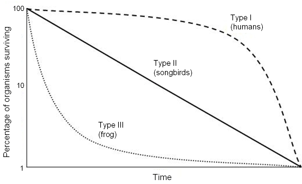
- Type I stays high through most of life, then drops steeply in old age: humans, orcas, whales and other large mammals with parental care.
- Type II declines at a steady rate (a constant proportion dies each year): many birds, some lizards, hydra.
- Type III drops steeply early, then flattens for the few survivors: corals, oysters, most fish with planktonic larvae, sea turtles (most hatchlings die, but survivors live long), many plants and insects. A seabird colony where most hatchlings die to predators and storms but survivors live for years also fits Type III.
A life table follows a cohort. Key columns: nₓ (alive at the start of age x), lₓ (proportion surviving to x), dₓ (dying during x), qₓ (death rate during x), and mₓ (offspring per individual at age x).
Age structure
Age structure diagrams (age pyramids) show the share of a population in each age class, often split by sex.
| Shape | Meaning |
|---|---|
| Broad base, narrow top (pyramid) | Many young: a growing (expanding) population |
| Straight sides, similar width (column) | Births roughly equal deaths: a stable population |
| Narrow base, wider middle or top (urn) | Few young: a declining population |
In fisheries, an age structure missing the oldest classes is a sign of overfishing, since fishing removes large, old fish first; a population missing its youngest classes signals recruitment failure (for example, from lost nursery habitat). Characteristics of a population include size, density, dispersion, age structure, sex ratio, and birth and death rates; an individual's phenotype is not a population characteristic.
Succession
Ecological succession is the gradual, fairly predictable change in a community's species over time.
- Primary succession starts on a surface with no soil or previous life: a new lava flow or volcanic island (corals settling on fresh volcanic rock), a newly exposed sandbar or mudflat, a sunken ship. Pioneer species (bacteria, cyanobacteria, algae, lichens on land; biofilms, algae and barnacles on rock in the sea) colonize first. r-strategists do well here.
- Secondary succession follows a disturbance that leaves soil, sediment or living remnants: a hurricane-flattened reef, a burned forest, a filled-in lake basin, a tsunami-scoured coast. It is faster than primary succession.
- The climax community is the relatively stable, self-sustaining end stage in equilibrium with the climate; in reality, disturbances often reset parts of it.
- Autogenic succession is driven by the organisms themselves changing the site (marsh plants trapping sediment and raising the ground); allogenic succession is driven by outside forces (sea-level change, sediment from a river, storms).
Salt-marsh succession (a halosere) shows both. One six-stage model describes it this way:
- Bare mud and colonization: algae and cyanobacteria film bare mudflats; their sticky mats start to trap sediment.
- Pioneer stage: salt-tolerant pioneers such as glasswort (Salicornia) and cordgrass (Spartina) germinate on the mud, slow the water and trap more sediment, raising the surface.
- Establishment: more seeds and spores arrive and grow; plant cover becomes continuous as the marsh builds up and is flooded less often.
- Competition: species diversity rises; less salt-tolerant plants (sea lavender, sea aster, then rushes) outcompete the pioneers.
- Stabilization: species settle into their niches and competition eases; the high marsh rarely floods.
- Climax: on ground no longer reached by the tides, shrubs and then woodland may take over.
Lakes undergo a parallel succession (a hydrosere): natural eutrophication and sediment slowly fill an aging lake, which becomes a marsh, then a meadow, then forest. Because the filled basin already has soil and seeds, the later stages are usually described as secondary succession.
On reefs, bare or recently killed coral is colonized first by turf and filamentous algae, then crustose coralline algae (which help coral larvae settle), and finally new corals. Heavy grazing pressure keeps the sequence moving toward coral; loss of grazers can stall it at fleshy algae.
Traditional ecological knowledge (Division C)
Traditional ecological knowledge (TEK), often called Indigenous knowledge, is the knowledge, practice and belief about local ecosystems that Indigenous and local communities build through long observation and pass between generations. It is place-based, often expressed through practice, story, song and ceremony, and frequently paired with rules about who may harvest what, where and when.
Coastal examples you can reason with:
- Hawaiian loko iʻa (fishponds) built with stone walls and sluice gates in estuaries and on reef flats let small fish in and kept grown fish from leaving; they depend on knowing tides, freshwater inflow and fish behavior.
- Ahupuaʻa were traditional Hawaiian land divisions running from mountain ridge to reef, managed as one watershed unit, which matches the modern idea of watershed (ridge-to-reef) management.
- Seasonal and area closures (for example kapu in Hawaiʻi, rāhui among Māori in New Zealand, and tabu areas or raʻui in other parts of the Pacific) rest a fishing ground or protect spawning times, which works like a modern marine protected area.
- Clam gardens on the Pacific Northwest coast of British Columbia and Washington: Indigenous peoples built rock walls at the low-tide line that flattened and extended the beach, creating more clam habitat. One study of these gardens found about four times as many butter clams and twice as many littleneck clams as on unmodified beaches.
- Salmon management by Pacific Northwest tribes: weirs were opened on schedule so enough fish passed upstream to spawn, and first-salmon ceremonies delayed the harvest until the run was established.
- Hazard knowledge: on Simeulue Island, Indonesia, an oral tradition (smong) taught people to run to high ground when the sea suddenly retreated; during the 2004 Indian Ocean tsunami, almost the whole island population survived. Moken sea nomads in Thailand and Myanmar also read the receding sea and fled.
- Local observation records, such as when a fish aggregates to spawn, when fish appear after ice melts, or where seagrass has retreated, can extend scientific monitoring back decades and set seasonal harvest timing.
Co-management shares decision-making between government agencies and Indigenous or local communities. In Washington State, the 1974 Boldt decision affirmed treaty tribes' right to half of the harvestable salmon and made tribes co-managers of the fishery with the state. The Mi'kmaq concept of Two-Eyed Seeing describes using the strengths of Indigenous knowledge with one eye and Western science with the other.
To apply TEK in a scenario, ask what long-term observations the community holds, what harvest rules they already follow, and how those can be combined with scientific data in co-management. Credit knowledge holders, involve them in decisions from the start (not just as consultants afterward), respect what they choose not to share, and treat TEK as evidence with its own methods, not as anecdote. TEK can also be combined with the population math above.
Applied issues: pollution, harmful species and watershed management
Part I gives scenarios, such as a fish kill, a closed shellfish bed or a town drinking contaminated water, and asks you to name the pollutant, trace where it came from, explain how it does harm and suggest a fix. This chapter sorts pollutants into types, follows them from the watershed to the sea, and covers the named examples that tests return to.
Types and sources of pollution
A pollutant is any substance or energy that makes water less fit for life or for human use. Sorting a pollutant into a type tells you how it does harm and how to stop it.
| Type | Examples | How it harms | Typical source |
|---|---|---|---|
| Oxygen-demanding (organic) wastes | Sewage, manure, food-processing waste, leaves | Decomposers use up DO (high BOD) | Sewage outfalls, feedlots, combined sewer overflows |
| Nutrients | Nitrate, ammonium, phosphate | Eutrophication, HABs, hypoxia | Fertilizer runoff, sewage, detergents, atmospheric N deposition |
| Pathogens | Bacteria, viruses, protozoa (Giardia, Cryptosporidium) | Disease; shellfish and beach closures | Sewage, septic leaks, animal waste, storm runoff |
| Sediment | Silt, clay, sand | Turbidity, smothering, carries P and toxins | Construction, farming, logging, bank erosion |
| Toxic inorganics | Mercury, lead, cadmium, arsenic, copper; acids | Poisoning, bioaccumulation | Mining, industry, coal burning, acid mine drainage |
| Toxic organics | Pesticides (DDT), PCBs, PAHs, oil | Poisoning, endocrine disruption, biomagnification | Industry, agriculture, spills, urban runoff |
| Thermal | Heated cooling water | Lowers DO, raises metabolism, thermal shock | Power plants and factories using once-through cooling |
| Radioactive | Radium, uranium, cesium, tritium | Radiation damage, cancer | Mining, nuclear accidents, natural deposits |
| Solid waste and plastics | Bags, bottles, fishing gear, microplastics | Entanglement, ingestion, carries other pollutants | Litter, stormwater, fishing, shipping |
| Emerging contaminants | PFAS, pharmaceuticals, personal-care products | Often long-term, low-dose effects | Wastewater, industry, firefighting foam |
Point source pollution enters from one identifiable place, such as a pipe, ditch or outfall: a sewage treatment plant, a factory discharge, or a power plant dumping heated water into a stream. Non-point source pollution comes from runoff spread over a large area: fields, lawns, parking lots, septic systems leaking across a whole shoreline, and air pollution settling on water. Point sources are easier to regulate (they can be permitted and monitored), which is why, since the Clean Water Act, nutrient loads from point sources have fallen sharply while non-point loads have not. The EPA names non-point source pollution as the leading remaining cause of water-quality problems in the U.S.
Sediment (siltation) has long been one of the most commonly reported pollutants of U.S. rivers and streams by miles impaired (pathogens now often rank first); for lakes and estuaries, nutrients are usually near the top of the list.
Not every waterborne pathogen comes from sewage. Vibrio bacteria (V. vulnificus, V. parahaemolyticus) live naturally in warm, brackish estuary water. They are concentrated by oysters and can cause severe illness from eating raw shellfish or through open wounds, and they are spreading poleward as water warms. Because they are not fecal, a low fecal coliform count does not prove shellfish are free of Vibrio; harvest rules in warm months also limit how long oysters can sit unrefrigerated.
Thermal pollution is a change in water temperature caused by people. The usual case is a power plant that takes in cool water, uses it to condense steam and returns it warmer. Warmer water holds less oxygen while animals need more, it can trigger thermal shock when the plant starts or stops, and it favors warm-water species and algae. Cooling towers and cooling ponds reduce it. Removing shade trees along banks and stormwater running off hot pavement also warm streams. Releases of cold bottom water from deep reservoirs are a form of thermal pollution too.
Acid rain forms when sulfur dioxide (SO₂) and nitrogen oxides (NOₓ) react in the air to form sulfuric and nitric acid. Coal-fired power plants are the main SO₂ source; vehicles and power plants produce NOₓ; ammonia from fertilizer and livestock adds nitrogen deposition. Limestone bedrock and soils neutralize acid (they add buffering), so a limestone mine is not a cause. Acid rain leaches calcium and magnesium from soils and releases toxic aluminum, which washes into streams and lakes; poorly buffered watersheds on granite are hit hardest, while lakes on limestone resist. Acid mine drainage forms when pyrite (FeS₂) in mine waste reacts with oxygen and water to make sulfuric acid (H₂SO₄) and dissolved iron, which precipitates as orange "yellow boy" (iron hydroxide) downstream.
Heavy metals: lead and mercury
Lead reaches drinking water mainly from inside the distribution system, not from the source: old lead service lines, lead solder and brass fixtures release it when the water is corrosive (low pH, low alkalinity, high chloride). Utilities prevent this with corrosion control, raising pH and adding orthophosphate, which forms a protective scale inside pipes. Lead is a neurotoxin with no known safe level, so the EPA's health goal (MCLG) is zero. In children it lowers IQ and causes learning problems, attention and behavior problems (including ADHD-like symptoms), slowed growth, hearing problems and anaemia; in adults it raises blood pressure and the risk of cardiovascular disease, damages the kidneys and harms reproduction. Lead is regulated by a treatment technique with an action level (15 ppb under the long-standing Lead and Copper Rule, lowered to 10 ppb by the 2024 Lead and Copper Rule Improvements, with compliance starting November 2027 and most lead service lines to be replaced within 10 years).
The Flint water crisis. In 2014, Flint, Michigan switched its supply from Detroit's treated Lake Huron water to the Flint River to save money, without adding corrosion-control treatment. The more corrosive river water stripped the protective scale from old pipes, and lead leached into tap water; blood-lead levels in children rose. The same period saw an outbreak of Legionnaires' disease. The city switched back in late 2015, and the crisis led to criminal charges, lead-pipe replacement and national attention on lead service lines.
Mercury comes mainly from coal burning (deposited from the air), mining and some industries. It is dangerous in water chiefly as methylmercury, which biomagnifies (see Bioaccumulation and biomagnification below) and damages the developing nervous system. Arsenic (natural in some groundwater, also from mine tailings and old pesticides) is regulated at an MCL of 10 µg/L (ppb) with an MCLG of zero; it causes skin lesions and cancers.
Salinization
Salinization is the build-up of dissolved salts in soils or fresh water. Causes include irrigation in dry climates (water evaporates and leaves its salts behind in the soil, and salty drainage returns to rivers), road de-icing salt washing into streams, lakes and groundwater, saltwater intrusion into coastal aquifers when wells pump too much fresh groundwater or the sea level rises, brines from mining and oil and gas wells, and clearing deep-rooted native vegetation, which lets salty groundwater rise. Rising salinity harms freshwater organisms that cannot osmoregulate in salty water, makes water unfit to drink or to irrigate crops, and corrodes pipes (releasing metals such as lead). Many rivers and lakes in the northern U.S. and Canada show steadily rising chloride from road salt.
Oil
Most oil reaching the ocean does not come from tanker disasters. In the U.S. National Research Council's estimates, natural seeps supply the largest share worldwide, and land runoff and routine discharges from ships and boats supply much of the rest; large spills are a small fraction of the total, though their local damage is severe.
| Spill | Year | Where | Key facts |
|---|---|---|---|
| Exxon Valdez | 1989 | Prince William Sound, Alaska | Tanker ran aground; about 11 million gallons; led to the Oil Pollution Act of 1990 (double hulls) |
| Deepwater Horizon | 2010 | Gulf of Mexico | Drilling-rig blowout; 11 workers killed; about 134 million gallons (3.19 million barrels, the 2015 court finding) to about 206 million gallons (4.9 million barrels, the federal government's estimate) over 87 days; the largest marine oil spill in U.S. history |
Oil harms by coating (feathers and fur lose insulation and waterproofing, so birds and otters die of hypothermia or drown), by toxicity (polycyclic aromatic hydrocarbons, PAHs, harm fish embryos), by smothering intertidal animals and marsh plants, and by blocking light and gas exchange at the surface. Response tools are booms to contain it, skimmers and sorbents to collect it, dispersants that break it into droplets, in-situ burning, and bioremediation (helping oil-eating bacteria).
Immediate versus long-term spill effects. In the first days and weeks, oil kills by coating (lost insulation and buoyancy), smothering and acute poisoning. Long-term effects can last years to decades: PAHs damage fish embryos and cause heart defects, reproduction and breeding fail (as in Prince William Sound herring after Exxon Valdez and Gulf dolphins after Deepwater Horizon), oil persists in marsh and beach sediments, and food webs shift as sensitive species decline.
How fast pesticides break down. Breakdown is usually first-order: a fixed fraction disappears per unit time, with rate constant . Many pesticides break down faster in sunlit water (photolysis and hydrolysis) than in soil, where they are shielded from light and bound to particles. Permethrin, for example, has a rate constant of roughly 0.025 per hour in the water column (half-life about a day) but a half-life of weeks in soil.
Tributyltin and imposex
Tributyltin (TBT) is an organotin biocide once used in antifouling paint on ship hulls to stop barnacles and algae from growing. It leached into harbors and marinas, where it is very toxic at parts-per-trillion levels. It acts as an endocrine disruptor: female snails such as dogwhelks develop male organs (imposex), which blocks breeding, and oysters grow thick, deformed shells (the classic case is Arcachon Bay, France, in the early 1980s). The U.S. restricted TBT paint on most small boats in 1988, and the International Maritime Organization's antifouling convention banned its use worldwide (no new application from 2003, none on hulls from 2008). It persists for years in harbor sediment, so dredging can release it again.
Bioaccumulation and biomagnification
Bioaccumulation is the build-up of a substance in one organism over its life, because it takes the substance in faster than it gets rid of it. Biomagnification is the rise in concentration from one trophic level to the next: each predator eats many prey and keeps their stored toxin. The substances that do this are persistent (not broken down), fat-soluble (stored in fatty tissue, not excreted in urine) and biologically active.
- Mercury: bacteria in low-oxygen sediments (especially sulfate-reducing bacteria) convert it to methylmercury, which biomagnifies in fish. Large predators (sharks, swordfish, king mackerel, tuna) carry the most. Minamata Bay, Japan (1950s) is the classic poisoning case.
- DDT: an insecticide that thinned eggshells of fish-eating birds (brown pelicans, ospreys, bald eagles); banned in the U.S. in 1972.
- PCBs: industrial insulating chemicals, banned in the U.S. in 1979; still in sediments and in the blubber of marine mammals.
- Ciguatoxin: made by the reef dinoflagellate Gambierdiscus; it passes from algae-grazing fish to predators such as barracuda, grouper, snapper and moray eels, so eating large reef predators causes ciguatera fish poisoning.
Watersheds and their management
A watershed (drainage basin, catchment) is all the land that drains to a common outlet: a stream, lake, estuary or the ocean. Its boundary is a divide, a ridge line from which water runs to different outlets. The Eastern Continental Divide along the Appalachians is why rain falling in West Virginia mostly flows west to the Ohio and Mississippi rivers while rain falling in much of Virginia flows east to the Chesapeake Bay. Everything done on the land shows up in the water, so a lake or estuary "reflects its watershed": the watershed supplies both its water and most of its pollutants.
- The Mississippi River watershed is the largest in the U.S., draining all or part of 31 states and 2 Canadian provinces, roughly 40% of the lower 48 states (about 1.2 million square miles). Its nutrients feed the Gulf of Mexico dead zone.
- The Chesapeake Bay watershed covers about 64,000 square miles in six states (Delaware, Maryland, New York, Pennsylvania, Virginia, West Virginia) and Washington, D.C.
- Small headwater streams make up most stream length in a watershed and process much of its nutrient and organic load, so what happens there matters a great deal downstream.
- An endorheic (closed) basin drains to an inland lake or sink with no outlet to the sea, such as the Great Salt Lake.
Urbanization replaces soil and plants with impervious surfaces (roofs, roads, parking lots). Less water soaks in, more runs off faster, peak floods rise, streams erode, groundwater recharge falls and runoff carries oil, metals, salt, heat and bacteria straight to the water.
Watershed management means managing land and water use across the whole basin to protect water quality and supply. Typical resource-management issues are accommodating growth while protecting water quality, balancing water for farms, cities, industry and ecosystems, controlling non-point runoff, protecting wetlands and fisheries, and supporting tourism without overloading the system.
Best management practices (BMPs) are practical measures that reduce runoff, erosion and pollutant loads. A strong answer names the pollutant and the step of its path that the BMP interrupts.
| BMP | What it does |
|---|---|
| Riparian buffer (vegetated strip along a stream) | Slows runoff, traps sediment, plant roots take up nutrients, shade keeps water cool; one of the most effective steps against diffuse nutrient loading |
| Cover crops | Hold soil and take up leftover nitrogen between cash crops |
| Conservation tillage (no-till), contour plowing, terracing | Reduce soil erosion from fields |
| Nutrient management | Apply fertilizer at the right rate, time and place |
| Controlled drainage and wetland restoration | Hold water so denitrification and settling can work |
| Livestock fencing | Keeps animals and manure out of streams |
| Retention/detention ponds, rain gardens, green roofs, permeable pavement | Capture urban stormwater and let it soak in or settle |
| Silt fences and sediment basins | Trap sediment on construction sites |
Applying fertilizer and manure so less washes off. Nutrient management follows the "4 Rs": the right source (type), right rate (no more than the crop needs, based on soil tests), right time and right place. In practice:
- Placement: fertilizer or manure injected below the surface or incorporated (tilled in) soon after spreading stays in the soil; fertilizer broadcast on the surface is the easiest for rain to wash away. Banding fertilizer near the roots also reduces losses.
- Timing: apply close to when the crop is actively growing, and not just before heavy rain or onto frozen, snow-covered or saturated ground, where it runs straight off. A rain right after a surface application washes the most nutrient into the nearest stream.
- Slope and distance: runoff is faster and carries more soil and fertilizer on steep slopes, so the highest risk is a steep field next to a stream with no buffer. Setbacks from water, contour farming and buffers cut this risk.
- Ammonium and nitrate fertilizers are very soluble: nitrate leaches to groundwater and drains, while phosphorus mostly travels attached to eroded soil.
Water conservation reduces demand. In agriculture, drip irrigation delivers water to the roots and loses far less to evaporation than sprinklers or flooding. Agriculture accounts for roughly 80% of U.S. consumptive water use (water withdrawn and not returned); by total withdrawals, irrigation and thermoelectric power cooling each take about 40%. At home, low-flow fixtures, fixing leaks and drought-tolerant landscaping (xeriscaping) help. Water reuse treats wastewater for irrigation or industry; California's Title 22 rules are state regulations that set treatment and bacteriological standards for recycled water and list the uses allowed for each level of treatment.
Pollution added along a river by many users (irrigation return flow, runoff from many towns and farms along a long river such as the Colorado) is classed as non-point source pollution, because no single outlet can be identified, even if each farm drain is small.
Climate change also changes behavior. Higher metabolic rates change how active fish are and how much they must eat; species shift where and when they feed and spawn; acidified water can impair some fishes' sense of smell and predator avoidance; and loss of coral or seagrass shelter changes habitat choice.
Water laws and agreements
| Law or treaty | Year | What it does |
|---|---|---|
| Clean Water Act (CWA) | 1972 | Goal of "fishable and swimmable" surface waters. Requires NPDES discharge permits for point sources (Section 402, the permit a sewage plant needs to discharge to a river or estuary); states list impaired waters and set TMDLs (total maximum daily loads) for them; Section 404 regulates dredging and filling of wetlands |
| Safe Drinking Water Act (SDWA) | 1974 | EPA sets standards for public drinking water. Primary standards (maximum contaminant levels, MCLs) protect health and are enforceable; secondary standards cover taste, odor and color and are guidelines only |
| Marine Protection, Research, and Sanctuaries Act (Ocean Dumping Act) | 1972 | Regulates dumping at sea; creates national marine sanctuaries |
| Coastal Zone Management Act | 1972 | Helps states manage coasts and estuaries |
| Oil Pollution Act | 1990 | Passed after Exxon Valdez; spill liability, response planning, double-hulled tankers |
| Ramsar Convention | 1971 | International treaty to conserve wetlands of international importance; the treaty specific to wetlands |
| National Estuary Program | 1987 | Clean Water Act amendment; EPA works with local partners on management plans for 28 "estuaries of national significance" (Chesapeake Bay has its own separate program) |
| National Estuarine Research Reserve System (NERRS) | 1972 law, first reserve 1974 | NOAA and coastal states run about 30 reserves for research, education and monitoring; its System-Wide Monitoring Program logs temperature, salinity, DO, pH, turbidity and more every 15 minutes |
| Magnuson–Stevens Act | 1976 | Manages U.S. fisheries in the 200-nautical-mile exclusive economic zone; requires ending overfishing and protecting essential fish habitat |
| Marine Mammal Protection Act | 1972 | Bans taking (hunting, harassing, killing) marine mammals in U.S. waters |
| Endangered Species Act | 1973 | Protects listed species and their critical habitat (e.g. elkhorn and staghorn corals, Nassau grouper) |
| MARPOL | 1973/1978 | International rules against pollution from ships, including oil and garbage |
| London Convention | 1972 | International treaty on dumping wastes at sea |
The EPA oversees tap-water quality under the SDWA. Water that meets every primary standard is considered safe to drink even if it fails a secondary standard (it may look, smell or taste bad, or stain fixtures).
| Drinking-water standard (EPA) | Value | Type |
|---|---|---|
| Nitrate (as N) | 10 mg/L | Primary (blue-baby syndrome) |
| Nitrite (as N) | 1 mg/L | Primary |
| Arsenic | 0.010 mg/L (10 ppb); goal (MCLG) zero because it is a carcinogen. Naturally high in bedrock wells of northern New England | Primary |
| Lead | Action level 15 ppb at the tap (10 ppb under the 2024 revisions, from November 2027); goal zero | Treatment technique |
| Copper | Action level 1.3 mg/L at the tap | Treatment technique |
| PFOA, PFOS | 4 parts per trillion each (2024 rule; compliance due 2029, which EPA proposed in 2026 to extend to 2031) | Primary |
| pH | 6.5–8.5 | Secondary |
| Iron | 0.3 mg/L | Secondary |
| Chloride | 250 mg/L | Secondary |
| Total dissolved solids | 500 mg/L | Secondary |
| Odor, color, taste | Limits set | Secondary |
For recreation, the EPA's 2012 criteria use E. coli (geometric mean 126 CFU per 100 mL) for fresh water and enterococci (35 CFU per 100 mL) for marine water. Older rules, still quoted in many tests, used fecal coliform at 200 per 100 mL for swimming. Shellfish-growing waters have a much stricter limit (a median or geometric mean of 14 fecal coliform per 100 mL under the national shellfish program), because shellfish concentrate bacteria.
Sedimentation
Sedimentation pollution is excess soil particles washed into water. Erosion from construction sites, cleared or overgrazed land, plowed fields, logging roads and collapsing stream banks sends silt and clay downstream; dredging and bottom trawling stir it back up; bottom-feeding fish and burrowing animals (bioturbation) resuspend it locally.
Effects follow from what the particles do:
- Block light → less photosynthesis by phytoplankton, seagrass and zooxanthellae → less food and oxygen.
- Smother → bury eggs, oyster beds, coral polyps and the gravel some fish spawn in; corals spend energy producing mucus to shed it.
- Harm fish directly: suspended sediment clogs and abrades gills, reduces resistance to disease, lowers growth rates, interferes with egg and larval development (silt fills the gaps in spawning gravel and suffocates eggs), and makes it harder for sight-feeding fish to find prey. It also smothers the bottom invertebrates fish eat. The same particles clog the feeding structures of filter feeders such as oysters and clams.
- Warm the water: dark suspended particles absorb sunlight and heat the water, which then holds less oxygen.
- Carry hitchhikers: phosphorus, metals, pesticides and bacteria stick to fine particles.
- Fill channels and harbors, which then need dredging.
Prevention works on the land: keep vegetation cover, plant riparian buffers and cover crops, avoid overgrazing, use silt fences and sediment basins on construction sites, and stabilize stream banks.
Harmful algal blooms
A harmful algal bloom (HAB) is a bloom of algae or cyanobacteria that harms people, animals or the ecosystem, either by making toxins or by sheer biomass (shading out seagrass, clogging fish gills, and using up oxygen when the bloom dies and decays). Marine HABs are mostly dinoflagellates and diatoms; freshwater and low-salinity HABs are mostly cyanobacteria ("blue-green algae", which are bacteria, not true algae). Red tides are usually dinoflagellate blooms, though not all red tides are toxic and not all HABs are red.
Blooms are favored by extra nutrients (nitrate and phosphate from fertilizer and sewage), warm water, sunlight, calm stratified water and slow flushing. HABs are a result of eutrophication, not its cause. People are exposed by eating shellfish or fish that concentrated the toxin, by swimming or skin contact, by breathing sea-spray aerosols (Florida red tide) and by drinking contaminated water.
| Organism (type) | Toxin | Illness or effect | Classic setting |
|---|---|---|---|
| Karenia brevis (dinoflagellate) | Brevetoxins | Neurotoxic shellfish poisoning; fish kills; airborne coughing and eye irritation | Florida "red tide," Gulf of Mexico |
| Alexandrium (dinoflagellate) | Saxitoxins | Paralytic shellfish poisoning (PSP) | Gulf of Maine, Pacific Northwest |
| Pseudo-nitzschia (diatom) | Domoic acid | Amnesic shellfish poisoning; sea lion and seabird poisonings | U.S. West Coast; first identified in Canada in 1987 |
| Dinophysis (dinoflagellate) | Okadaic acid | Diarrhetic shellfish poisoning | Many temperate coasts |
| Gambierdiscus (dinoflagellate, lives on algae and dead coral) | Ciguatoxins | Ciguatera fish poisoning from eating large reef fish | Tropical reefs; toxin biomagnifies |
| Pfiesteria (dinoflagellate) | Disputed toxin | Fish kills with skin lesions | North Carolina and Chesapeake estuaries, 1990s |
| Microcystis (cyanobacterium) | Microcystins | Liver damage; drinking-water bans | Lake Erie: Toledo's 2014 "do not drink" order, driven by farm phosphorus |
| Dolichospermum (formerly Anabaena) (cyanobacterium) | Anatoxins, others | Nerve toxins; dog deaths | Lakes and reservoirs |
Shellfish beds are closed during blooms because filter feeders concentrate the toxins, and cooking does not destroy them. Agencies monitor with water samples (cell counts), toxin tests on shellfish, and satellite images of chlorophyll. HAB toxins can force "do not drink" advisories because ordinary treatment and boiling do not reliably remove them.
Know the bloom-forming groups. Diatoms are single-celled algae with glass-like cell walls (frustules) of silica, so blooms draw down dissolved silicate; they reproduce fast and are classic r-selected producers. Dinoflagellates have two flagella and many have cellulose plates; some are photosynthetic, some eat other cells, and some (zooxanthellae) live inside corals. Cyanobacteria are photosynthetic bacteria; many fix nitrogen in special cells called heterocysts, which lets them thrive where nitrogen is scarce and warm water favors them. Trichodesmium is a nitrogen-fixing marine cyanobacterium that forms "sea sawdust" blooms in the tropics.
Harmful species
The words overlap, so define them carefully:
- Native species belong in the area. A native species can still become harmful when the system is out of balance (crown-of-thorns outbreaks, coral-eating Drupella snails).
- Non-native (exotic, introduced, nonindigenous) species were moved by people outside their natural range. Most are harmless.
- Invasive species are non-native species that spread and cause ecological, economic or health harm.
- Aquatic nuisance species is the U.S. legal term (from the 1990 Nonindigenous Aquatic Nuisance Prevention and Control Act) for nonindigenous aquatic species that threaten native species or ecosystems, or human uses such as fishing, recreation, water supply and industry. "Nuisance" is also used for native species that grow out of control.
Invaders succeed because they leave behind the predators, parasites, diseases and competitors that held them in check at home (the "enemy release" idea), and because many grow fast, reproduce early, eat many foods and tolerate a wide range of conditions. They harm by eating natives, outcompeting them for food or space, spreading disease, interbreeding with natives, changing habitat, and clogging pipes and intakes. Invasive populations often show boom-and-bust dynamics: explosive growth followed by a crash.
Pathways: ship ballast water (ships take on water to stay stable when empty and release it, with any larvae, at the next port), hull fouling, aquarium and pet releases, escapes from aquaculture and fish farms, live bait, and canals linking basins. Escaped farmed salmon, for example, compete with and interbreed with wild fish and spread disease and sea lice.
Management follows the invasion curve: prevention is cheapest, then eradication while a population is small, then containment, and finally long-term management of an established species. Boaters help with clean, drain, dry: remove plants and animals from the boat, drain all water, and dry gear before moving to another water body.
| Species | Native to | How it arrived | Harm | Notes and control |
|---|---|---|---|---|
| Lionfish (Pterois volitans, P. miles) | Indo-Pacific | Aquarium releases off Florida (first records in the 1980s) | Eats many small reef fish and juveniles; few predators; venomous spines | Spearfishing, derbies, promoting it as food |
| Zebra mussel (Dreissena polymorpha) | Caspian and Black Sea region | Ballast water; Great Lakes, 1988 | Clogs water intakes; outcompetes native mussels; filters out plankton (clearer water, less food) | Largely replaced in the Great Lakes by quagga mussels |
| Asian carp (bighead, silver, grass, black) | East Asia | Escaped from aquaculture ponds in the southern U.S. | Outcompete natives for plankton; silver carp leap at boats | Electric barriers near Chicago, commercial harvest, renamed "copi" to sell as food |
| Spiny water flea | Eurasia | Ballast water | Eats zooplankton, altering plankton communities | Spread by fishing lines and boats |
| Sea lamprey | Atlantic | Through shipping canals into the Great Lakes | Parasitizes lake trout and other fish | Lampricides and barriers |
| European green crab | Europe | Ballast water, ship fouling | Eats clams and young oysters; damages eelgrass | Trapping |
| Chinese mitten crab | East Asia | Ballast water | Burrows into banks causing erosion; clogs intakes | San Francisco Bay |
| Asian shore crab | Western Pacific | Ballast water | Competes with native crabs on Atlantic shores | Very abundant from Maine to North Carolina |
| Caulerpa taxifolia ("killer algae") | Tropical seas | Aquarium strain escaped in the Mediterranean | Smothering mats crowd out seagrass | Eradicated from a California lagoon by covering and chlorinating |
| Orange cup coral (Tubastraea) | Indo-Pacific | Ship hulls and oil platforms | Competes with native Caribbean and Gulf corals | — |
| Nutria | South America | Fur farming releases | Eats marsh plant roots, turning marsh to open water (Chesapeake, Louisiana) | Trapping and bounty programs |
| Water hyacinth | South America | Ornamental plant | Dense floating mats block light, lower DO, block boats | Fast-growing nuisance plant |
| Hydrilla, Eurasian watermilfoil | Asia; Eurasia | Aquarium and boat trade | Dense submerged mats | Common invasive aquatic plants in North America |
| Purple loosestrife, common reed (Phragmites australis, non-native strain) | Eurasia | Ornamental; ballast soil | Take over wetlands and marsh edges | Biocontrol beetles for loosestrife |
| Giant salvinia | South America | Aquarium and water-garden trade | Floating fern mats cover Texas and Louisiana lakes | Spotted gar, by contrast, is a native fish |
| Northern snakehead | East Asia | Live-food markets, releases | Top predator in Potomac and Chesapeake tributaries | Air-breathing; can survive out of water |
| Green mussel (Perna viridis) | Indo-Pacific | Ballast water, hull fouling | Fouls intakes, buoys and oyster reefs in Florida | Warm-water invader of the U.S. Southeast |
| Overbite clam (Potamocorbula amurensis) | East Asia | Ballast water, San Francisco Bay, 1986 | Filters so much plankton that it cut phytoplankton and the food supply of native fish | One reason San Francisco Bay has few large blooms |
| Snowflake coral (Carijoa riisei) | Western Atlantic | Hull fouling into Hawaii | Smothers native black corals and reef invertebrates | Octocoral; a reef invader |
| Invasive red algae (Kappaphycus, Gracilaria, Acanthophora) | Indo-Pacific and elsewhere | Imported for seaweed farming or by hull fouling, Hawaii | Overgrow and smother Hawaiian reef flats | Removed with underwater vacuums ("Super Sucker") and native urchin restocking |
| Carpet sea squirt (Didemnum vexillum) | Probably Northwest Pacific | Hull fouling, aquaculture gear | Colonial tunicate mats smother scallop and gravel beds (Georges Bank) | — |
| Dead man's fingers (Codium fragile) | Northwest Pacific | Shellfish transport, hull fouling | Green alga that displaces kelp and fouls shellfish beds in New England | — |
Recently killed coral
Reef surveys sort the bottom into categories, and recently killed coral is one of them: coral that has died within about the past year, with the skeleton still white or lightly fuzzed and the polyp structure still visible, before algae fully cover it. It is a snapshot of recent stress. A rise in recently killed coral after a heat wave points to bleaching mortality; patches with feeding scars point to crown-of-thorns or snail predation; a broken, scattered pattern points to storms, anchors or blast fishing.
Emerging contaminants
Emerging contaminants are chemicals now being detected in water whose effects are not fully understood or regulated. Conventional treatment plants were not designed to remove most of them.
PFAS (per- and polyfluoroalkyl substances) are a family of thousands of synthetic chemicals with chains of carbon–fluorine bonds, among the strongest bonds in chemistry. That is why they repel water and grease, and why they almost never break down ("forever chemicals"). They are used in nonstick cookware, stain- and water-resistant fabrics and carpets, grease-proof food packaging, and aqueous film-forming firefighting foam (AFFF), which has contaminated groundwater around airports and military bases. Industrial plants can release them too; GenX, made along North Carolina's Cape Fear River, contaminated the drinking water of downstream towns. PFAS travel easily in water, cross into groundwater and bioaccumulate, binding to proteins in blood and liver.
Health effects linked to PFAS exposure in EPA summaries include higher cholesterol, liver damage (changed liver enzymes), weaker vaccine response and other immune effects, thyroid disease, high blood pressure in pregnancy, lower birth weight, and higher risk of kidney and testicular cancer. Symptoms are usually not obvious; the harm shows up as raised risks over time.
In 2024 the EPA set the first enforceable drinking-water limits for PFAS, including 4 parts per trillion each for PFOA and PFOS. In 2025–2026 the EPA said it would keep the PFOA and PFOS limits but proposed extending their compliance deadline from 2029 to 2031 and rescinding the 2024 limits for PFHxS, PFNA, GenX and a PFAS mixture. Removing PFAS takes granular activated carbon, ion-exchange resins or high-pressure membranes (reverse osmosis, nanofiltration); boiling does not remove them.
Other emerging contaminants:
- Pharmaceuticals and personal-care products pass through people and wastewater plants. Some are endocrine disruptors, which mimic or block hormones: synthetic estrogen from birth-control pills has caused intersex fish, with males producing the egg-yolk protein vitellogenin.
- Microplastics are plastic pieces smaller than 5 mm: primary ones made small (microbeads, banned from rinse-off cosmetics in the U.S. by the Microbead-Free Waters Act of 2015, pellets, fibers shed from clothing) and secondary ones broken from larger plastic by sunlight and waves. They are eaten by plankton, filter feeders and fish, and they carry absorbed toxins.
- Sunscreen chemicals such as oxybenzone and octinoxate can harm coral larvae; Hawaii banned their sale from 2021.
- Flame retardants and other industrial chemicals that persist and bioaccumulate.
The five ocean garbage patches
The five major subtropical gyres, in the North Pacific, South Pacific, North Atlantic, South Atlantic and Indian Ocean, are huge rotating current systems that collect floating debris into garbage patches. The best known is the Great Pacific Garbage Patch in the North Pacific Gyre between Hawaii and California. The patches are not solid islands: they are a thin "soup" of mostly small plastic pieces and microplastics spread through the upper water, with larger items such as nets scattered through it, and they move and change shape with the currents. Abandoned, lost or discarded fishing gear, called ghost gear or ghost nets, makes up a large share of the mass of the Great Pacific Garbage Patch and keeps catching and entangling fish, turtles, mammals and corals ("ghost fishing").
About 80% of marine pollution, including most marine debris, is commonly estimated to come from land (litter carried by rivers, storm drains and wind); the rest comes from fishing, shipping and offshore platforms. Plastic harms by entanglement, ingestion (animals mistake it for food and starve with full stomachs; sea turtles eat bags that look like jellyfish), carrying invasive species on floating debris, absorbing and concentrating persistent pollutants, and smothering reefs and seabeds. Cleanup is hard because the pieces are tiny and dispersed over enormous areas, nets that collect plastic also catch plankton and animals, and new plastic keeps arriving; cutting inputs at the source (reducing single-use plastic, better waste management, recovering fishing gear) does the most good.
Climate change and other pressures on estuaries
Climate change acts on every part of the event:
- Warming: lower oxygen solubility, stronger stratification, more hypoxia, coral bleaching, more frequent HABs and cyanobacteria blooms, and species shifting their ranges toward the poles or into deeper water. Spawning, migration and bloom timing shift too.
- Sea-level rise: marshes and mangroves drown if they cannot build up or move inland; salt water pushes farther up estuaries and into coastal aquifers (saltwater intrusion).
- Acidification: lower pH and aragonite saturation (see pH and aragonite saturation).
- Acidification in estuaries: river water carries little alkalinity, and respiration in nutrient-rich bottom water adds CO₂, so estuaries can reach low pH and low aragonite saturation sooner than the open ocean. From 2007 to 2009, Pacific Northwest oyster hatcheries lost most of their larvae when upwelled, CO₂-rich water with low Ω entered their intakes; hatcheries now monitor carbonate chemistry and buffer the water.
- Deoxygenation: the ocean as a whole is losing oxygen as it warms.
- Stronger storms and changing rainfall: pulses of fresh water, sediment and nutrients.
Other human threats to estuaries are draining and filling wetlands for development, dredging channels, building dams that cut river flow and sediment supply and block fish migration, shoreline hardening (seawalls), overfishing, pollution and invasive species.
Water treatment
Two separate systems handle water for people. Drinking-water (potable) treatment makes source water safe to drink; wastewater treatment cleans used water before it returns to a river or estuary. Learn the stages in order and the purpose of each.
Potable water
A typical surface-water plant runs these steps:
- Screening and intake: bar screens remove sticks, fish and debris.
- Pre-treatment: aeration strips dissolved gases (hydrogen sulfide, carbon dioxide) that cause odor and corrosion and oxidizes dissolved iron and manganese so they can be removed; some plants pre-oxidize with chlorine, ozone or permanganate.
- Coagulation: a coagulant is mixed in rapidly. Alum (aluminum sulfate, Al₂(SO₄)₃) is the most common; ferric chloride, ferric sulfate and polyaluminum chloride are alternatives. Tiny colloidal particles (roughly 0.001 to 1 µm: clay, bacteria, color-causing organics) carry negative surface charges, so they repel each other and never settle. The coagulant supplies positively charged ions (Al³⁺, Fe³⁺) that neutralize those charges so the particles can stick together. Coagulant aids (polymers, called polyelectrolytes) help bind the particles into stronger flocs. Colloids are so small that the random jostling of water molecules (Brownian motion) keeps them suspended indefinitely, which is why gravity alone cannot remove them. Coagulants work only within a pH and alkalinity window, so plants often add lime (calcium hydroxide) or soda ash to supply alkalinity; lime is also used in lime softening to precipitate the calcium and magnesium that cause hardness. In choosing a coagulant, operators weigh the raw water's pH and alkalinity, its temperature (cold water slows floc formation), the amount and type of turbidity, the volume of sludge produced, and cost and availability. A jar test (several beakers of raw water dosed with different amounts, stirred and allowed to settle) finds the best dose.
- Flocculation: slow, gentle mixing lets the destabilized particles collide and grow into large, heavy flocs. Mixing too hard breaks them up.
- Sedimentation (clarification): water sits in basins so flocs settle by gravity; the process relies on the particles being denser than water. If particles are not settling, likely causes are flocs that are too small or light (wrong coagulant dose or pH, too-cold water), flow that is too fast or short-circuits through the basin, mixing that breaks flocs, density or temperature currents, or wind.
- Filtration: water passes through sand, anthracite coal and gravel (rapid sand or dual-media filters) or membranes to remove the remaining fine particles and many microbes. Filters are cleaned by backwashing. Slow sand filters rely on a biological layer (schmutzdecke) on top of the sand. Activated carbon adsorbs taste, odor and organic chemicals.
- Disinfection: kills remaining pathogens (details below).
- Finishing: pH and corrosion control (to keep lead and copper from leaching from pipes), fluoridation (0.7 mg/L is the U.S. Public Health Service recommended level as of October 2026; HHS began reviewing it in 2025), sometimes softening, then storage and distribution with a disinfectant residual.
The memory order is coagulation → flocculation → sedimentation → filtration → disinfection. Coagulation, flocculation and sedimentation remove suspended solids together; filtration polishes; disinfection targets microbes.
| Disinfectant | How it works | Advantages | Drawbacks |
|---|---|---|---|
| Chlorine (gas, hypochlorite) | Strong oxidant | Cheap; leaves a residual that keeps protecting water in the pipes; most widely used | Forms disinfection byproducts (trihalomethanes, haloacetic acids) with organic matter; weak against Cryptosporidium |
| Chloramine (chlorine + ammonia) | Weaker, longer-lasting oxidant | Stable residual in long pipe networks; fewer byproducts | Slower; toxic to aquarium fish and dialysis patients unless removed |
| Ozone (O₃) | Very strong oxidant, made on site | Kills Cryptosporidium and viruses; removes taste and odor | No residual; costly; highly corrosive, so contact tanks and pipes must be corrosion-resistant (stainless steel) |
| Ultraviolet light | Damages microbial DNA so cells cannot reproduce | No chemicals; effective against Cryptosporidium and Giardia | No residual; needs clear water, since turbidity shields microbes |
Desalination turns seawater or brackish water into fresh water. Reverse osmosis forces water through a semipermeable membrane at pressures above the osmotic pressure, leaving salts behind; it is now the most widely used method. Distillation (multi-stage flash and multi-effect) boils water and condenses the vapor, which is very pure because dissolved salts do not evaporate. Electrodialysis uses an electric field and ion-selective membranes and suits brackish water. All produce concentrated brine that must be disposed of, and all use a lot of energy. Dry, wealthy coastal nations such as Saudi Arabia, the United Arab Emirates, Kuwait and Israel depend heavily on it.
Slow sand filters need no chemicals or electricity: water percolates slowly through sand topped by a biological film (schmutzdecke) that traps and digests microbes and organic matter. They clog quickly in turbid water, so very turbid water must be pretreated (settled or roughing-filtered) first.
Boiling at home. When a utility issues a boil-water advisory (after a main break or loss of pressure), the purpose is to kill pathogens. The CDC calls a rolling boil for 1 minute (3 minutes above about 6,500 ft) the surest way to kill bacteria, viruses and parasites; boiling does not remove chemicals such as lead, nitrate or PFAS, and can concentrate them.
Wastewater
Sewage treatment removes solids, organic matter (BOD), nutrients and pathogens in stages. The raw wastewater entering the plant is the influent; the treated water leaving it is the effluent.
- Preliminary treatment: bar screens remove rags and large objects (some plants instead use a comminutor, which grinds solids small enough to pass on); a grit chamber lets sand and gravel settle so they do not wear out pumps. Fats, oils and grease (FOG) are skimmed early because they clog pipes and coat equipment.
- Primary treatment (physical): in a primary clarifier heavier solids settle as sludge and fats and oils are skimmed. It removes roughly half of the suspended solids and about a third of the BOD.
- Secondary treatment (biological): microbes eat dissolved and fine organic matter. In activated sludge systems air is bubbled into an aeration basin so aerobic bacteria consume organic matter; the microbes then settle in a secondary (final) clarifier, and part of that sludge is returned to keep the process seeded. Trickling filters (water trickles over rocks or plastic media coated with a microbial film), rotating biological contactors and lagoons do the same job. Secondary treatment removes most of the BOD; the U.S. standard is about 85% removal (30 mg/L BOD₅ and TSS, monthly average).
- Tertiary (advanced) treatment: extra steps where the receiving water is sensitive or the water will be reused. Examples: nitrogen removal by nitrification (aerobic, ammonia → nitrate) followed by denitrification (in low-oxygen, anoxic tanks with a carbon source, bacteria use nitrate instead of oxygen and release N₂ gas; oxygen must be kept out, or the bacteria use it instead); phosphorus removal by chemical precipitation (alum or iron salts) or biological uptake; filtration of fine particles; activated carbon to remove micropollutants. Tertiary treatment is not only biological.
- Disinfection before discharge: chlorine (then dechlorination, because chlorine residue harms aquatic life) or UV.

Sludge from the clarifiers is thickened, then usually anaerobically digested, which stabilizes it, kills many pathogens and produces biogas (mostly methane) that can power the plant. It is then dewatered and disposed of or applied to land as biosolids: treated sewage sludge that meets EPA standards for pathogens and metals. In the U.S., about 60% of sewage sludge (EPA's 2024 estimate) is land-applied as fertilizer and soil conditioner on farms, forests, reclaimed mine land and lawns; most of the rest goes to landfills, and a smaller share is incinerated. Concern is growing because biosolids can carry PFAS and other persistent chemicals onto fields. Trace the water and the sludge as two separate paths when a diagram asks you to order stages. Constructed wetlands can provide polishing treatment for small communities.
Combined sewer systems, found in many older U.S. cities (about 700 communities), carry sewage and stormwater in the same pipes. In heavy rain the flow exceeds plant capacity and the excess discharges untreated as a combined sewer overflow (CSO), sending bacteria, nutrients and debris into rivers and estuaries. That is why fecal coliform counts spike after storms. Separate storm sewers, storage tunnels and green infrastructure reduce CSOs.
Industrial pretreatment. Factories that send waste to a city plant must pretreat toxic substances first (the EPA pretreatment program under the Clean Water Act), because metals and toxic organics can kill the microbes that run secondary treatment, contaminate sludge so it cannot be used as biosolids, and pass straight through the plant into the river or estuary.
Preliminary or primary? Many textbooks and answer keys fold screening and grit removal into primary treatment. If "preliminary" is not an option, removal of large debris is part of primary treatment.
Septic systems
Homes without sewers use a septic system. Wastewater flows into a buried septic tank, where solids settle into a sludge layer, grease and oils float as a scum layer, and anaerobic bacteria partly digest the solids. The liquid in the middle flows out to a drainfield (leach field) of perforated pipes in gravel, where it soaks into the soil; soil microbes and filtering finish the treatment.
| Failure | Cause | Fix |
|---|---|---|
| Clogged drainfield | Tank never pumped, so solids escape into the field; grease and wipes flushed | Pump the tank every 3–5 years; keep grease, wipes and chemicals out |
| Hydraulic overload | Too much water at once (laundry loads, leaks, roof drains) | Spread out water use, fix leaks, divert roof and surface water |
| Poor soil percolation or high water table | Clay soils or saturated ground cannot absorb effluent, so sewage surfaces | Proper site testing; mound or alternative systems |
| Physical damage | Roots, vehicles driving over the field, cracked tank | Keep trees and vehicles off; inspect and repair |
Failing septic systems near estuaries leak bacteria and nutrients, so they are a common cause of shellfish-bed closures and nitrogen loading.
Coral reefs
Part II is worth 30% of the score. It has two halves: reef ecology (coral biology, reef types, zones, threats, health indicators, management) and the 23 listed indicator organisms. Tests ask both "what is it" questions (identify a photo, give a scientific name, name a phylum) and "why" questions (why does a falling parrotfish count matter, why does nutrient runoff lead to crown-of-thorns outbreaks). This chapter covers both. Water chemistry behind reefs (pH, carbonate, aragonite saturation Ω) is in pH and aragonite saturation. Eutrophication in general is in Eutrophication, and invasive species such as lionfish are in Harmful species.
Coral biology
What a coral is
A coral is an animal, not a plant or a rock. Corals belong to phylum Cnidaria, the group that also contains sea anemones, jellyfish and hydroids. All cnidarians share four features that tests ask about:
- Radial symmetry (body parts arranged around a central axis).
- Cnidocytes, stinging cells. Each holds a harpoon-like capsule, the nematocyst, that fires on contact.
- A gastrovascular cavity with a single opening that is both mouth and anus.
- Two possible body forms: the attached polyp and the swimming medusa (jellyfish). Corals and anemones (class Anthozoa) live only as polyps and have no medusa stage.
Within Anthozoa, two subclasses matter for the list:
| Group | Tentacles | Skeleton | Reef builder? | List example |
|---|---|---|---|---|
| Hexacorallia: stony corals (order Scleractinia) | Smooth, in multiples of 6 | Hard external aragonite skeleton | Yes, the main framework builders | Hard/stony corals |
| Octocorallia: soft corals, sea fans, sea whips | Exactly 8, feathery (pinnate) | Flexible protein (gorgonin) axis and/or tiny calcite sclerites in the tissue | No (blue coral Heliopora is the exception, with a massive aragonite skeleton) | Gorgonia sea fans |
A few other organisms also add limestone to reefs: fire corals (Millepora, actually hydrozoans, not true corals), blue coral and organ-pipe coral (octocorals), crustose coralline algae (red algae that cement the reef), the green alga Halimeda (its plates become sand), and tube-building worms and molluscs.
Hermatypic corals are reef-building corals. Most of them are zooxanthellate, fast-calcifying and colonial. Ahermatypic corals do not build reefs. Most are solitary or form small colonies and lack zooxanthellae, so they can live in dark or deep water.
Polyp anatomy
A stony coral polyp is a soft sac a few millimeters across (some solitary species reach several centimeters), sitting in a cup of its own skeleton.

Work through the diagram from top to bottom.
| Part | What it is and does |
|---|---|
| Tentacles | Ring around the mouth; armed with nematocysts; catch zooplankton, mostly at night |
| Nematocyst | Stinging capsule inside a cnidocyte; also used in fights with neighboring corals |
| Mouth | Single opening; food in, wastes and gametes out |
| Pharynx | Short tube from the mouth into the gut |
| Gastrovascular cavity | Gut space where digestion starts; divided by radial mesenteries |
| Mesenterial (digestive) filaments | Edges of the mesenteries; secrete enzymes; can be pushed out through the mouth or body wall to digest prey or attack rival corals |
| Epidermis (outer layer) | Outer cell layer; holds cnidocytes |
| Mesoglea | Jelly-like middle layer between the two cell layers |
| Gastrodermis | Inner cell layer lining the gut; this is where the zooxanthellae live, inside the cells |
| Calicoblastic epidermis | Bottom layer of the polyp, touching the skeleton; secretes the aragonite |
| Coenosarc | Living tissue sheet connecting neighboring polyps across the colony surface |
| Corallite | Skeletal cup of one polyp; its wall is the theca, its radial ridges are septa, its central pillar is the columella, its floor is the basal plate |
| Coenosteum | Skeleton laid down between corallites, under the coenosarc |
Corals compete for space in three ways: they grow faster or overtop rivals and shade them out; they extend long sweeper tentacles loaded with nematocysts; and they push out mesenterial filaments to digest a neighbor's tissue.
Zooxanthellae and coral nutrition
Zooxanthellae are single-celled dinoflagellates (protists, not plants and not diatoms) that live inside the gastrodermis cells of reef-building corals. They used to be placed in one genus, Symbiodinium. Since 2018 the group has been split into several genera in the family Symbiodiniaceae (for example Symbiodinium, Breviolum, Cladocopium and the relatively heat-tolerant Durusdinium). One square centimeter of coral tissue holds on the order of a million cells. The relationship is mutualism, and an endosymbiosis because the alga lives inside the host's cells.
| The coral gives the algae | The algae give the coral |
|---|---|
| A protected place in the light (corals grow toward the sun) | Up to about 90% of the coral's energy needs (commonly cited; estimates run as high as 95% in bright shallow water) |
| CO₂ from respiration | Organic products of photosynthesis: glucose, glycerol, amino acids, fatty acids and other lipids. Passing these to the host is called translocation |
| Nitrogen (ammonium) and phosphate wastes | Oxygen |
| Faster calcification ("light-enhanced calcification"): photosynthesis removes CO₂ and supplies energy for building skeleton | |
| Most of the brown, green or golden color of healthy coral |
This tight swap explains how reefs thrive in nutrient-poor water: nutrients are recycled between animal and alga instead of being lost. Corals are still mixotrophs: at night polyps extend their tentacles and catch zooplankton, and they also absorb dissolved organic matter and trap particles in mucus. Heterotrophic feeding supplies nitrogen and phosphorus the algae cannot provide, and it matters most for deeper corals and during bleaching.
Other animals on the list also farm zooxanthellae: giant clams keep them in their mantle, and many gorgonians host them too. Coral reef food webs therefore have two kinds of primary producers: the zooxanthellae inside animals, and free-living algae (turf, fleshy macroalgae, coralline algae and phytoplankton).
Reproduction and growth
Corals reproduce both sexually and asexually.
Sexual reproduction. Most reef-building corals are hermaphrodites (each polyp makes both eggs and sperm); others have separate male and female colonies.
- Broadcast spawners (the majority of reef-building species) release eggs and sperm, often packaged in buoyant egg–sperm bundles, into the water. Fertilization is external at the surface. On the Great Barrier Reef, mass spawning happens a few nights after a full moon in late spring (October to December); in Florida and the Caribbean, in late summer (August to September), a few nights after the full moon, an hour or more after sunset. Synchrony swamps egg predators and raises the chance that sperm meets eggs of the same species. The floating spawn can form pink-red slicks that wash onto beaches.
- Brooders release only sperm. Eggs are fertilized inside the parent polyp, and well-developed larvae are released later, often over several months. Brooded larvae settle quickly and near the parent.
- Fertilized eggs develop into a planula larva: a free-swimming, ciliated, pear-shaped larva. It drifts for days to weeks, then settles on clean hard substrate, often cued by crustose coralline algae. It metamorphoses into a single primary polyp, secretes a basal plate and starts its skeleton.
Asexual reproduction builds and spreads colonies:
- Budding: a polyp divides or sprouts a new polyp. Division inside the ring of tentacles (intratentacular budding) without full separation produces the long meandering valleys of brain coral. Budding is how one primary polyp becomes a colony of thousands of genetically identical polyps.
- Fragmentation: broken branches (from storms, for example) reattach and grow. Branching corals such as Acropora rely heavily on this. Coral restoration uses the same process.
- Less common: polyp bail-out (polyps leave a stressed colony and resettle) and parthenogenesis (larvae from unfertilized eggs).
So the full cycle runs spawning → fertilization → planula larva → settlement → primary polyp → budding into a colony (a test may also call the last step "cloning").

Growth rates. Corals grow slowly, and growth form matters. Massive (boulder and brain) corals add roughly 0.3–2 cm per year. Branching corals such as staghorn and elkhorn can add about 10 cm per year, sometimes up to 20 cm. Whole reefs accrete vertically only millimeters per year, because bioeroders (parrotfish, boring sponges, urchins) and storms remove much of what corals build. Some colonies are centuries old.
Reef types and formation
Reef geologists classify reefs by their shape and their position relative to land.
| Type | Shape and position | Lagoon? | Examples |
|---|---|---|---|
| Fringing reef | Grows seaward directly from the shore of a continent or island; the youngest and most common type | None, or a very narrow, shallow back-reef channel | Red Sea coasts, much of the Caribbean, Hawaiian islands |
| Barrier reef | Runs parallel to the shore but separated from it by a wide, often deep lagoon | Yes, between reef and land | Great Barrier Reef (Australia), Mesoamerican (Belize) Barrier Reef, New Caledonia, the Florida Reef Tract |
| Atoll | A ring or horseshoe of reef, often topped by low sandy islets, around a central lagoon with no central island | Yes, central | Maldives, Marshall Islands (Enewetak, Kwajalein), Tuamotus |
| Patch reef | Small, isolated outcrop, usually inside a lagoon or on a shelf; needs no nearby dry land | Surrounded by sand or lagoon floor | Patch reefs in the Florida Keys and in atoll lagoons |
| Platform (bank) reef | Grows on a shallow offshore platform and can grow outward in all directions | Sometimes a small one | Many reefs of the outer Great Barrier Reef shelf |
Darwin's subsidence theory (1842) links the first three types into one sequence. A fringing reef grows around a young volcanic island. As the island slowly subsides (sinks as the cooling crust beneath it contracts and the volcano erodes), the reef keeps growing upward to stay in the light, so a lagoon opens between reef and shore: a barrier reef. When the island has sunk completely, only the ring of reef remains: an atoll. Drilling at Enewetak Atoll in the early 1950s went through more than 1.2 km of reef limestone before hitting volcanic basalt, which confirmed the idea. Later work added sea-level change: during ice ages sea level fell by over 100 m, exposing and eroding reefs, which then regrew when the sea rose again. So treat Darwin's sequence as the standard model for volcanic islands, not the only way reefs form (continental-shelf barrier reefs such as the Great Barrier Reef did not form around a sinking volcano).

Where the big reef systems are
- Indo-Pacific: by far the most reef area and the most species. The Coral Triangle (Indonesia, Malaysia, the Philippines, Papua New Guinea, Timor-Leste and the Solomon Islands) holds about 76% of the world's reef-building coral species and the highest reef fish diversity.
- Great Barrier Reef, off Queensland, Australia: the largest reef system, about 2,300 km long, made of roughly 2,900 individual reefs and some 900 islands.
- Mesoamerican Barrier Reef (Mexico, Belize, Guatemala, Honduras), including the Belize Barrier Reef: the second-largest reef system, in the western Caribbean.
- Florida Reef Tract: the only extensive shallow reef system in the continental United States, a bank-barrier reef along the Florida Keys.
- Atlantic/Caribbean reefs are mostly fringing and barrier reefs and have far fewer species than the Indo-Pacific: roughly 60–70 Caribbean stony coral species versus several hundred in the Coral Triangle.
- Deep cold-water reefs: Lophelia pertusa (now Desmophyllum pertusum) builds reefs at roughly 200–1,000 m in 4–12 °C water with no zooxanthellae, feeding on plankton. Examples are off Norway (the Røst Reef is the largest known; the Tisler Reef is noted for yellow colonies) and off the southeastern United States. The main threat is bottom trawling, which smashes colonies centuries old.
- Mesophotic reefs (about 30–150 m) are light-dependent reefs below normal diving depth. They get less UV and less wave and heat stress, which is one reason they are proposed as refuges.
Where reefs grow: physical requirements
Every requirement follows from two facts: the zooxanthellae need light, and the coral needs to precipitate aragonite.
| Factor | What reefs need | Why |
|---|---|---|
| Temperature | About 18–30 °C; best growth roughly 23–29 °C; most reefs lie between about 30° N and 30° S | Below about 18 °C calcification is too slow; a few weeks at 1 °C above the usual summer maximum causes bleaching |
| Light and depth | Clear water; most reef growth in the upper 25–30 m, with zooxanthellate corals reaching about 100 m or more in very clear water | Photosynthesis of the zooxanthellae; reefs lie in the neritic (coastal, over the continental shelf) photic zone |
| Water clarity (turbidity) | Low turbidity and low sedimentation | Sediment blocks light and smothers polyps; corals spend energy cleaning themselves with mucus |
| Salinity | Full-strength seawater, about 32–40 (often quoted as 32–38 ppt); reefs are absent near large river mouths | Low salinity (floods, runoff) or high salinity stresses corals and can trigger bleaching |
| Nutrients | Low nitrate and phosphate (oligotrophic water) | Extra nutrients favour fast-growing algae and phytoplankton that shade and overgrow corals and feed crown-of-thorns larvae |
| Substrate | A solid, hard surface for larvae to attach to | Planulae cannot settle on mud or shifting sand |
| Water movement | Moderate waves and currents; high dissolved oxygen | Delivers plankton and oxygen, removes sediment and wastes; strong waves build the reef crest |
| Carbonate chemistry | Aragonite saturation Ω above about 3; best above about 4 (Ω 3–3.5 is marginal) | Ω controls how easily aragonite precipitates; see pH and aragonite saturation |
Reefs also grow best on the western sides of ocean basins (the Caribbean, western Pacific, western Indian Ocean), where warm currents flow poleward, and are scarce on the eastern sides (west Africa, western South America), where cold, nutrient-rich upwelling dominates. That is why there are no reefs off California or Peru at the same latitudes. Storm protection is not a requirement; reefs grow in hurricane belts.
Reef zones and reef fish communities
A reef profile from shore to open sea passes through zones with different wave energy, light and organisms. On a fringing reef there may be little or no back reef.
| Zone (shore to sea) | Setting | Typical life |
|---|---|---|
| Lagoon / back reef | Closest to shore, sheltered behind the crest; calm, sandy floor, warmer and more variable | Patch reefs, seagrass, sea cucumbers, sand-dwelling fish, juvenile fish; giant clams and Diadema in the Indo-Pacific |
| Reef flat | Shallow platform just behind the crest; may be exposed at very low tide | Hardy corals, turf algae, urchins, snails |
| Reef crest (on many Indo-Pacific reefs an algal ridge) | The highest point of the reef, where waves break; highest energy | Crustose coralline algae, wave-resistant corals such as elkhorn coral in the Caribbean |
| Fore reef (reef front, reef face, reef slope) | Seaward slope below the crest; may have spur-and-groove (buttress) ridges and channels, then a drop-off | Highest coral and fish diversity: many coral growth forms, sponges, gorgonians, groupers, snappers, sharks |
| Deep fore reef / off-reef floor | Below the main coral zone | Plate-shaped corals that spread to catch dim light, sponges, sand |
Reef fish communities. A reef supports hundreds of fish species in a small area, divided by diet, time of day and microhabitat:
- Herbivores: parrotfish, surgeonfish, rabbitfish and damselfish crop algae. With urchins they keep space open for coral settlement.
- Corallivores: many butterflyfish and some parrotfish eat coral tissue or mucus.
- Planktivores: damselfish, anthias and fusiliers feed in the water column above the reef.
- Invertebrate feeders: sweetlips and grunts, many wrasses, triggerfish.
- Piscivores and apex predators: groupers, snappers, jacks, barracuda, moray eels and reef sharks.
- Cleaners: cleaner shrimp (including the banded coral shrimp) and cleaner wrasses run "cleaning stations".
Day and night shifts are sharp. By day, butterflyfish, parrotfish and damselfish are active and colorful; at dusk they shelter in crevices, and nocturnal species emerge: moray eels, snappers, sweetlips and grunts, squirrelfish, lobsters, Diadema urchins, and coral polyps opening to feed. Most nocturnal reef fish are predators (carnivores), which is one reason daytime visual counts can underestimate them. Many reef fish are flattened from side to side, an adaptation for turning quickly among branches and slipping into crevices.
Coral reef fish diversity is high partly because larval supply is unpredictable. The lottery hypothesis holds that when space opens up, whichever species' larvae arrive first take it, so no species can exclude the rest by competition.
Why reefs matter
Commonly cited numbers (expect these exact figures on tests):
| Fact | Commonly cited value |
|---|---|
| Area | Less than 1% of the ocean floor; often given as about 0.1% (some sources say "less than a quarter of one percent") of the ocean |
| Biodiversity | About 25% of all marine species (also stated as 25% of marine fish species) depend on reefs at some stage; called the "rainforests of the sea" |
| People | Hundreds of millions of people (often "half a billion" or about 1 billion) depend on reefs for food, income or coastal protection |
| Economic value | Hundreds of billions of US dollars per year worldwide (NOAA has long cited about 2.7 trillion for all reef goods and services) |
| Wave protection | A healthy reef can absorb up to about 97% of incoming wave energy |
| Largest reef system | Great Barrier Reef |
Ecosystem services:
- Habitat and nursery for fish and invertebrates, including commercially fished species.
- Fisheries and food security, especially for island nations.
- Coastal protection: reefs break waves and reduce erosion and storm-surge flooding; artificial seawalls are costlier and less effective.
- Tourism and recreation: diving, snorkeling, fishing.
- Medicines: reef organisms are rich in bioactive compounds. Nucleosides from a Caribbean sponge led to the anticancer drug cytarabine (Ara-C), and a sponge compound led to the breast-cancer drug eribulin.
- Sand and land: parrotfish and Halimeda produce much of the white carbonate sand of reef beaches and islands; atolls are made entirely of reef.
What harms reefs
Threats are often split into natural and anthropogenic (human-caused). Natural: cyclones and hurricanes, crown-of-thorns outbreaks (although humans make them worse), disease, El Niño heat, extreme low tides, predation. Anthropogenic: everything else below. The two worst global threats are warming (bleaching) and changing ocean chemistry (acidification).
| Threat | Mechanism and effect | Typical signs in a survey |
|---|---|---|
| Warming / bleaching | Heat plus strong light break the coral–algae partnership; corals starve and die | White but intact corals, then recently killed coral |
| Ocean acidification | CO₂ dissolves → carbonic acid → fewer carbonate ions → lower Ω → slower calcification, weaker skeletons, faster dissolution | Slower growth (seen in long-term records, not in one survey) |
| Overfishing | Removes herbivores (algae take over) and predators (food web imbalance; crown-of-thorns and urchin outbreaks) | Few large fish, small average size, missing groupers, snappers, parrotfish |
| Blast (dynamite) fishing | Explosives stun or kill fish and shatter the reef into rubble | Craters, rubble fields, few fish |
| Poison (cyanide) fishing | Cyanide squirted into crevices stuns fish for the live food fish and aquarium trades; kills corals and small animals | Missing humphead wrasse, barramundi cod, large groupers; bleached patches |
| Bottom trawling, dredging | Weighted nets or dredges flatten reef structure; dredging cuts channels through reefs | Rubble, broken colonies; main threat to deep Lophelia reefs |
| Nutrient pollution (sewage, fertilizer) | Feeds fleshy algae and phytoplankton; more food for crown-of-thorns larvae; can promote disease | High nutrient indicator algae |
| Sedimentation (land clearing, construction, dredging) | Blocks light, smothers polyps and larvae, prevents settlement | Silt on the bottom, turbid water |
| Chemical pollution | Oil, pesticides, heavy metals; sunscreen chemicals oxybenzone and octinoxate harm coral larvae and promote bleaching at low concentrations | Coral damage near outfalls or crowded beaches |
| Disease | Bacterial, cyanobacterial and fungal infections; worse with heat and pollution | Bands or patches of dead tissue |
| Crown-of-thorns outbreaks (Indo-Pacific) | Thousands of starfish strip live coral | White feeding scars, recently killed coral |
| Invasive species | Indo-Pacific lionfish in the western Atlantic since the mid-1980s eat small reef fish; orange cup coral (Tubastraea) spreads on Caribbean hard surfaces | Lionfish counts, cup coral on reefs and rigs |
| Collection | Aquarium trade (fish, shrimp, corals), curio trade (shells, urchins, coral skeletons), coral mining for building blocks and lime | Missing collected species, mined patches |
| Tourism and boats | Anchors, groundings, divers' fins and hands, trampling, coastal development | Broken colonies, scars, trash |
| Storms | Cyclones break and overturn colonies; dead structure is then taken over by macroalgae | Rubble, broken colonies |
Coral bleaching
Coral bleaching is the loss of zooxanthellae (or of their pigment) from coral tissue. The coral turns pale or white because the white skeleton shows through the now-transparent tissue. The coral is not dead at that point.
Mechanism. Under high temperature combined with strong light, the zooxanthellae's photosynthetic machinery is damaged and produces reactive oxygen species (ROS) such as superoxide, hydrogen peroxide and hydroxyl radicals. These damage both partners, and the coral expels or digests its symbionts. The coral then starves: it loses most of its energy supply, stops growing and reproducing, and becomes more susceptible to disease. If the stress ends within weeks, the coral can regain symbionts from the few that remain and recover over months. If it lasts, the coral dies and algae colonize the skeleton.
Causes. Most often, and behind all the mass bleaching events, it is water warmer than the usual summer maximum. Other triggers: unusually cold water, very high light or UV (calm, clear, low-tide days), low salinity after floods, sediment, pollutants (including sunscreen chemicals), nutrient imbalance, disease and exposure at low tide.

Measuring heat stress: NOAA Coral Reef Watch. NOAA's Coral Reef Watch uses satellite sea-surface temperature to track bleaching risk for every reef.
- HotSpot: how far the current temperature is above the maximum monthly mean (MMM), the long-term average temperature of the warmest month.
- Degree Heating Weeks (DHW): accumulated heat stress, the sum of HotSpots of at least 1 °C over the past 12 weeks, in °C-weeks. One week at 1 °C above the MMM is 1 DHW. Three weeks at 1 °C above is 3 DHW, and so is one week at 3 °C above.
- Alert levels: 4 DHW → Bleaching Alert Level 1, significant bleaching likely. 8 DHW → Alert Level 2, severe, widespread bleaching and significant mortality likely. In 2023 NOAA added Levels 3–5 (12, 16 and 20 DHW) for increasingly severe mortality risk; Level 5 means risk of near-complete (over 80%) coral death.
Global bleaching events. NOAA recognizes four global events: 1998 (tied to a strong El Niño), 2010, 2014–2017 (the longest; the Great Barrier Reef bleached severely in 2016 and again in 2017, and in 2018 new coral recruitment there was about 89% below historical levels according to a 2019 Nature study, a drop often summarized as "80–90%"), and 2023–2025, the fourth event, declared in April 2024 (NOAA said in 2026 that it likely ended in mid-2025). By April 2025 bleaching-level heat stress had reached about 84% of the world's reef area in more than 80 countries and territories, the largest on record. Back-to-back bleaching years are especially damaging because corals have no time to recover between them.
Coral diseases
Coral diseases are usually named after the band or pattern of tissue loss they leave. They spread faster in warm, polluted water.
| Disease | Cause | Notes |
|---|---|---|
| Black band disease | A mat of cyanobacteria (originally named Phormidium corallyticum, now Roseofilum reptotaenium) with sulfide-producing bacteria | A dark band moves across the colony, leaving bare white skeleton; worse in warm, nutrient-rich water |
| White band disease | Bacterial (exact agent uncertain) | Tissue peels off from the base of Acropora branches; with heat and storms it destroyed most Caribbean elkhorn and staghorn coral from the late 1970s on, and both species are now Critically Endangered |
| White plague | Bacterial | Fast tissue loss on massive corals |
| White pox | Linked to Serratia marcescens, a bacterium from human sewage | Irregular white patches on elkhorn coral in the Florida Keys |
| Yellow band (yellow blotch) | Bacterial (Vibrio) | Yellow bands on star corals |
| Stony coral tissue loss disease (SCTLD) | Probably bacterial, possibly involving the symbionts; spreads by contact and water | First seen off Miami in 2014; now in much of the Caribbean; affects more than 20 stony coral species and kills colonies within weeks to months; treated with antibiotic paste |
| Aspergillosis | Fungus Aspergillus sydowii | Kills sea fans (Gorgonia), causing purple lesions; Caribbean-wide outbreaks in the 1990s |
Crown-of-thorns outbreaks
The crown-of-thorns starfish (COTS) is a native Indo-Pacific coral predator. At normal densities it is part of the ecosystem. During an outbreak, densities rise from about one per hectare to hundreds or thousands, and they can strip a reef of most of its live coral; outbreaks are one of the main causes of coral loss on the Great Barrier Reef. Each adult can eat up to about 10 m² of coral per year, and a large female can release tens of millions of eggs in a season (estimates reach about 200 million).
Two hypotheses, which are not mutually exclusive, explain outbreaks:
- Nutrient enrichment (larval starvation hypothesis): runoff after heavy rain fuels phytoplankton blooms. COTS larvae feed on phytoplankton, so many more survive.
- Predator removal: overfishing of COTS predators (giant triton, humphead wrasse, some groupers, emperors, triggerfish and pufferfish) lets more young starfish survive.
Control: divers inject each starfish with a single shot of bile salts (ox bile) or household vinegar (acetic acid), approved on the Great Barrier Reef; both kill it within a day or two without harming other reef life. Older methods used multiple injections of sodium bisulfate or simply removing the starfish by hand. Cutting starfish up does not work because the pieces can survive and regenerate. Long-term control means reducing runoff and protecting predators.

Managing reefs
Management reduces local stresses so reefs can better survive the global ones.
| Tool | What it does |
|---|---|
| Marine protected areas (MPAs) | Limit damaging activities in an area; the common goal is to rebuild fish populations, which then spill over into surrounding fished waters |
| No-take zones (marine reserves) | Ban all fishing; the strongest recovery of large predators and herbivores. About a third of the Great Barrier Reef Marine Park has been no-take "green zones" since 2004 |
| Locally managed marine areas (LMMAs) | Communities set their own closures and rules, often using traditional knowledge (common in the Pacific) |
| Fishery rules | Size limits, catch quotas, gear bans (no blast or cyanide fishing, no trawling near reefs, no spearfishing with scuba), protection of herbivores such as parrotfish, closed seasons and protection of spawning aggregations (for example of the Nassau grouper) |
| Trade controls | CITES Appendix II listings for stony corals, giant clams and the humphead wrasse require export permits; aquarium-collection licenses |
| Water quality | Cut fertilizer and sediment runoff, upgrade sewage treatment, protect mangroves and seagrass that trap sediment |
| Tourism controls | Mooring buoys instead of anchors, diver education, limits on visitors; sunscreen rules (Hawaii passed the first US ban on sunscreens containing oxybenzone and octinoxate in 2018, in force from 2021) |
| Direct intervention | COTS culling by injection; lionfish removal and derbies; treating SCTLD lesions with antibiotics |
| Restoration | Coral gardening: fragments are grown in underwater or land-based nurseries (asexual reproduction by fragmentation) and outplanted; microfragmentation speeds growth of massive corals; collecting spawn to raise and settle larvae; breeding heat-tolerant corals; re-establishing grazers such as Diadema |
| Monitoring | NOAA Coral Reef Watch (satellite heat stress and bleaching alerts), Reef Check (volunteer surveys), the Global Coral Reef Monitoring Network, AGRRA (Caribbean rapid assessments) |
| Addressing climate change | Cutting CO₂ emissions is the only fix for warming and acidification |
Individuals help by choosing sustainable seafood, using reef-safe sunscreen, not touching or collecting reef life, not buying coral or shell curios, cutting energy use and plastic, and supporting protected areas.
Reef health indicators and Reef Check surveys
The 2027 handout names five reef health indicators. Know what each one measures and what a change in it means.
| Indicator | What is measured | Healthy reef | Degraded or overfished reef |
|---|---|---|---|
| Marine apex predators | Presence and numbers of sharks, large groupers, snappers, jacks | Present and common; on remote unfished reefs predators can make up most of the fish biomass | Rare or absent; their loss lets mid-level predators and coral eaters increase |
| Biomass | Total weight of fish per area (kg per hectare), from counts and estimated lengths | High | Low; a falling fish biomass signals declining reef health |
| Average catch length | Mean size of fish in catches or surveys | Large fish, many big breeding adults | Falling mean length: fishers remove the largest fish first, a classic sign of overfishing |
| Coral cover | Percentage of the bottom covered by live hard coral | High, often 30–50% or more on good reefs | Low coral cover with more algae, rubble and recently killed coral; Caribbean average coral cover fell from about 50% in the 1970s to about 10% by the early 2000s |
| Indicator organisms | Counts of the 23 listed organisms | Diverse, with large individuals | Missing species point to the specific pressure (see grouping tables below) |
Reef Check is a volunteer reef-monitoring program founded in 1996 by marine scientist Gregor Hodgson. Divers trained as "EcoDivers" use one standard protocol worldwide, so data can be compared across countries. A standard survey:
- Site: lay a 100 m transect tape along a depth contour, usually at two depths: shallow (about 2–6 m) and mid-reef (about 6–12 m).
- Segments: four 20 m segments separated by 5 m gaps (0–20, 25–45, 50–70 and 75–95 m), so each depth has four replicates.
- Fish belt transect: after laying the line the diver waits a few minutes for fish to return, then swims each segment counting indicator fish in a belt 5 m wide (2.5 m either side of the line) and 5 m high. Groupers are counted with size classes (only those over 30 cm); parrotfish only over 20 cm.
- Invertebrate belt transect: the same 5 m × 20 m belts, searched closely (including crevices) for indicator invertebrates. Coral damage (bleaching, disease, anchor and blast damage) and trash are also recorded.
- Substrate line (point-intercept) transect: the diver records what lies directly under the tape every 0.5 m, 40 points per segment and 160 per depth.
| Code | Substrate category | What it tells you |
|---|---|---|
| HC | Hard coral (live stony coral, including bleached coral, fire coral and organ-pipe coral) | Coral cover |
| SC | Soft coral | Live cover |
| RKC | Recently killed coral (dead within about the past year; white or lightly fuzzed, coral structure still sharp) | Recent mortality: bleaching, COTS, disease, blasting |
| NIA | Nutrient indicator algae (fleshy macroalgae taller than turf) | Nutrient pollution and loss of grazers |
| SP | Sponge | Filter feeders; can increase on degraded reefs |
| RC | Rock (hard bottom, including coral dead more than a year and covered in turf or crusts) | Older mortality; also suitable surface for settlement |
| RB | Rubble (loose coral fragments) | Storms, blast fishing, anchors |
| SD | Sand | Natural bottom type |
| SI | Silt/clay | Sedimentation |
| OT | Other sessile organisms (anemones, tunicates, zoanthids, Halimeda) | Background |
Belt counts convert to density in the same way. Each 5 m × 20 m segment is 100 m², so 4 segments cover 400 m². Six parrotfish over 20 cm across all four segments is 6 ÷ 400 m² = 1.5 per 100 m².
The 2027 organism list
The 2027 Coral Reef Ecology handout lists 23 indicator organisms: 15 global (found in both the Indo-Pacific and Atlantic regions), 5 Indo-Pacific only and 3 Atlantic only. The list is based on the Reef Check worldwide indicator list. Reef Check chose organisms that are easy for volunteers to recognize and that respond to particular human pressures: fishing pressure (including destructive blast and cyanide fishing), collection for the aquarium and curio trades, and nutrient pollution. Their absence, or the absence of large individuals, points to a specific pressure.
How it is tested:
- Identification: picture matching by common name (the 2027 sample tournament matched photos of eight organisms: parrotfish, moray eel, hard coral, crown-of-thorns starfish, grouper, banded coral shrimp, butterflyfish and pencil urchin). Learn each organism by sight from the gallery below.
- Names and classification: matching scientific names (Acanthaster planci, Epinephelus striatus), naming the family (Serranidae, Scaridae), picking the phylum ("which is NOT an echinoderm"), and region ("Tridacna spp.: Indo-Pacific only").
- Ecology: diet, predators, reproduction (sex change, spawning aggregations), behavior (cleaning, mucus cocoons), role in the reef (keystone grazer, bioeroder), and why surveys count it.
Indicator organism reference
The table follows the handout order within each region. "Status" is the IUCN Red List category where the species has been assessed. Use it to answer feeding, life-cycle and "why counted" questions, then use the grouping tables after it to answer "which one is NOT" questions.
ReferenceCoral reef indicator organisms· 23 rows
IUCN categories: LC least concern, NT near threatened, VU vulnerable, EN endangered, CR critically endangered, DD data deficient. COTS = crown-of-thorns starfish.
No rows match.
| Organism (scientific name) | Region | Group (phylum; class) | How to recognize it | Feeding | Reproduction and life cycle | Ecology and behavior | Why surveys count it / threats | Status |
|---|---|---|---|---|---|---|---|---|
| Banded coral shrimp (Stenopus hispidus) | Global (circumtropical; Atlantic, Indian and Pacific) | Arthropoda; Malacostraca (Crustacea, Decapoda) | Small (body about 5–6 cm) shrimp with red and white bands; enlarged, banded third pair of legs ending in claws; very long white antennae | Cleaner: picks parasites, dead tissue and fungus off fish, including morays; also scavenges | Separate sexes; lives in monogamous pairs, the female is larger than the male; female carries green eggs under her abdomen; planktonic larvae | Waits at a cleaning station in a crevice, waving antennae to attract fish; mutualism (fish lose parasites, shrimp gets food); pairs defend territory | Aquarium trade (popular, easily collected) | Not assessed |
| Butterflyfish (Chaetodon spp.; family Chaetodontidae) | Global | Chordata; Actinopterygii | Thin, disc-shaped body; small protruding mouth with brush-like teeth; usually a dark bar through the eye and often an eyespot near the tail; no spine on gill cover (angelfish have one) | Many are corallivores (eat coral polyps and mucus); others eat small invertebrates, algae or plankton | Many form long-term pairs; pelagic spawners (buoyant eggs drift); larvae have a tholichthys stage with bony head plates; young are called fry | Diurnal and colorful by day, shelter in crevices at night with duller colors; closely related to angelfish | Aquarium trade; corallivores decline when live coral is lost, so they track reef health ("canary of the reef"); they take little tissue and rarely spread coral disease | Most species LC |
| Crown-of-thorns starfish (Acanthaster planci) | Global on the handout; in reality Indo-Pacific only, from the Red Sea to the eastern Pacific (no Atlantic COTS) | Echinodermata; Asteroidea | Large (often 25–35 cm, rarely up to about 60–80 cm) sea star with many arms (about 7–23) covered in long, sharp, venomous spines; gray, purple, red or green | Corallivore: climbs onto coral, everts its stomach over it and digests the tissue, leaving white skeleton; prefers fast-growing branching corals such as Acropora | Separate sexes; broadcast spawner, females release millions to tens of millions of eggs (up to about 200 million a year in large females); larvae feed on phytoplankton for weeks; juveniles eat coralline algae before switching to coral | Normally hides by day; outbreaks of hundreds to thousands of starfish strip reefs | Outbreaks follow nutrient runoff (better larval survival) and loss of predators (triton, humphead wrasse, some fish); controlled by injecting bile salts or vinegar | Not assessed; now treated as a complex of four species (Pacific populations are A. solaris) |
| Fleshy algae (red Rhodophyta, green Chlorophyta, brown Phaeophyta) | Global | Not animals: red and green algae (Archaeplastida), brown algae (Stramenopiles; Phaeophyceae) | Soft, upright seaweeds taller than turf (canopy over about 1–3 cm); e.g. Dictyota, Lobophora, Sargassum (brown), Caulerpa (green), Laurencia (red); calcified Halimeda and crustose coralline algae are not "fleshy" | Producers (photosynthesis); pigments: red algae phycoerythrin, green algae chlorophylls a and b, brown algae fucoxanthin | Sexual and asexual (fragments regrow); grow fast | Food for herbivores and habitat for small animals; but they compete with coral for light and space, overgrow and shade corals, carry coral-killing microbes and block larval settlement | Recorded as nutrient indicator algae: high cover means nutrient pollution and/or loss of grazers (overfishing of parrotfish, urchin die-off); a phase shift away from coral | Not assessed |
| Grouper >30 cm (Serranidae, subfamily Epinephelinae) | Global | Chordata; Actinopterygii | Heavy body, big mouth with projecting lower jaw, rounded or straight tail; many spotted or barred; can change color; large species exceed 1 m and 100 kg (goliath grouper over 2 m) | Ambush predators of fish, crustaceans and octopus; suck in and swallow prey whole (few cutting teeth) | Most are protogynous hermaphrodites (mature as females, some later become males); many form spawning aggregations at fixed sites and moon phases | Slow growing, long lived, late maturing; territorial; some hunt cooperatively with moray eels; large groupers prey on morays | Overfishing, spearfishing, live reef food fish trade (often caught with cyanide); only fish over 30 cm are counted because fishing removes big ones first | Varies; about 1 in 8 grouper species is threatened |
| Hard / stony corals (order Scleractinia) | Global | Cnidaria; Anthozoa (Hexacorallia) | Rigid aragonite skeleton made of many cups (corallites); growth forms branching (staghorn, elkhorn), massive (brain, boulder), plate, encrusting; fire coral is counted as HC in Reef Check but is a hydrozoan | Mixotroph: up to about 90% of energy from zooxanthellae, plus zooplankton caught at night with nematocyst tentacles | Broadcast spawning or brooding → planula → polyp → budding into a colony; fragmentation | The reef framework; habitat for most other reef life | Live coral cover is the basic health measure; lost to bleaching, disease, COTS, sediment, blasting, anchors, mining | 44% of reef-building coral species assessed as threatened (IUCN, 2024); Caribbean elkhorn and staghorn CR |
| Lobsters (Nephropidae as printed; on reefs mostly spiny lobsters, Palinuridae) | Global | Arthropoda; Malacostraca (Crustacea, Decapoda) | Clawed lobsters (Nephropidae, e.g. Homarus) have big front claws and live mainly in cool water. Spiny lobsters (Panulirus) have no large claws, very long thick spiny antennae and a spiny shell | Nocturnal omnivores and scavengers: snails, clams, crabs, urchins, worms, carrion and algae; eat their own moulted shell to recover calcium | Separate sexes; female carries eggs under the tail ("berried"); spiny lobster larvae (phyllosoma) drift for months; grow by moulting | Hide in dens by day; spiny lobsters rasp their antennae to make a warning sound and migrate in single-file queues; red pigment astaxanthin becomes visible when cooked because heat frees it from the protein that masks it | Overfishing (valuable food species); trap and dive fisheries | Mostly LC or DD |
| Long-spined black sea urchins (Diadematidae; Diadema spp.) | Global (D. antillarum Atlantic; D. setosum, D. savignyi Indo-Pacific) | Echinodermata; Echinoidea | Black (juveniles banded) urchin with very long, thin, hollow, brittle spines (often 10–30 cm); test about 10 cm; mildly venomous | Herbivore: grazes turf and fleshy algae at night using Aristotle's lantern (five-toothed jaw); also scrapes some coral | Separate sexes; broadcast spawner; planktonic larvae; slow recovery because larvae must arrive from elsewhere | Keystone grazer in the Caribbean: keeps algae down and opens space for coral settlement; too many can overgraze and bioerode the reef; shelters in crevices by day; small fish shelter among spines | Indicates grazing balance and overfishing of its predators (triggerfish, wrasses); 1983–84 Caribbean die-off killed over 93–99% of individuals, followed by algal takeover; 2022 die-off caused by a Philaster scuticociliate | Not assessed |
| Moray eel (Muraenidae) | Global | Chordata; Actinopterygii | Long, scaleless, snake-like body covered in mucus; no pectoral (side) fins; continuous dorsal fin; usually only the head shows from a crevice | Nocturnal predator of fish, octopus, crabs and shrimp; uses a second set of pharyngeal jaws that shoots forward to pull prey into the throat | Pelagic spawning; leaf-shaped transparent leptocephalus larvae drift for months | Opens and closes its mouth constantly to pump water over the gills (not aggression); cleaned by cleaner shrimp; some hunt cooperatively with groupers; preyed on by large groupers, sharks, barracuda | Overfishing and aquarium trade; some cause ciguatera if eaten | Most species LC |
| Parrotfish >20 cm (Scaridae; now often placed within the wrasse family Labridae) | Global | Chordata; Actinopterygii | Large scales, teeth fused into a parrot-like beak; often blue-green and pink; terminal-phase males are brightly colored, initial-phase fish (mostly females) duller and look like different species | Herbivores: scrape epilithic algae (turf on dead coral) and some live coral; pharyngeal teeth grind the limestone, which comes out as sand | Most are sequential (protogynous) hermaphrodites: females can become terminal-phase males; pelagic spawners, often in groups | Many sleep in a mucus cocoon secreted from glands in the gill cavity, which may hide their scent from predators and keep off blood-feeding parasites; a large parrotfish can produce hundreds of kilograms of sand per year, much of the white sand on reef beaches; grazing is mostly non-lethal to coral | Overfishing, especially night spearfishing of sleeping fish; loss of parrotfish leads to algal overgrowth; only fish over 20 cm are counted | Most species LC |
| Pencil urchins (Eucidaris spp.; Indo-Pacific slate pencil urchin Heterocentrotus also seen) | Global (E. tribuloides western Atlantic, E. thouarsii eastern Pacific, E. metularia Indo-Pacific) | Echinodermata; Echinoidea | Few thick, blunt, pencil-like spines, often coated with algae, sponges and coralline crusts; Eucidaris test about 5 cm (spines spread wider); Heterocentrotus has huge triangular red spines | Omnivorous grazer: algae, encrusting invertebrates, bryozoans, sponges and some coral, bitten off with Aristotle's lantern | Separate sexes; broadcast spawner; planktonic larvae | Nocturnal; wedges into crevices by day with its heavy spines, which also helps in strong currents | Curio collection (spines and tests used in jewelry and wind chimes) and aquarium trade | Not assessed |
| Snapper (Lutjanidae) | Global | Chordata; Actinopterygii | Elongate body, sloping triangular head, large mouth with canine teeth, slightly forked tail; red, yellow or silver; school by day | Carnivores: fish, crustaceans, octopus and other invertebrates; many hunt at night; do not eat coral | Separate sexes; many form spawning aggregations; pelagic eggs and larvae; juveniles often use mangroves and seagrass as nurseries | Mid- to upper-level predators | Overfishing (major food fish); some large species cause ciguatera | Most LC; a few VU (e.g. cubera snapper) |
| Demosponges (Demospongiae) | Global | Porifera; Demospongiae | Sessile; tubes, vases, barrels, fans or crusts; many small pores (ostia) and a few large openings (oscula); bright colors; the largest sponge class (over 80% of sponge species) | Filter feeders: flagellated choanocytes pump water through the body and trap bacteria and fine particles; also absorb dissolved organic matter | Mostly hermaphrodites; sperm released, eggs often fertilized inside and released as swimming larvae (so juveniles are not stationary); asexual by budding, fragmentation and gemmules; strong regeneration from fragments | Skeleton of spongin (a collagen protein; the reason some are used as bath sponges) and/or silica spicules; no muscles, nerves or true tissues; chemical defenses (toxins, bad taste) deter predators, though hawksbill turtles and angelfish eat them; boring sponges (Cliona) erode coral; recycle dissolved organic matter into food for reef animals; giant barrel sponge lives centuries | Habitat and water filtration; sponges often increase on degraded or nutrient-rich reefs; sources of medicines (cytarabine); glass sponges (another class) dominate polar and deep water | Mostly not assessed |
| Sweetlips (Haemulidae; Plectorhinchus spp. in the Indo-Pacific) | Global as a family; Plectorhinchus is mainly Indo-Pacific; on Atlantic reefs the family is represented by grunts (Haemulon) | Chordata; Actinopterygii | Thick, fleshy lips; adults spotted or striped; juveniles look completely different (blotched, colorful) | Nocturnal bottom feeders: crabs, shrimp, bristle worms, molluscs | Separate sexes; pelagic spawners | Rest in groups under ledges by day; juveniles live alone in shallow water and swim with an exaggerated undulating wriggle, apparently mimicking toxic flatworms or nudibranchs; the family makes grunting sounds by grinding its pharyngeal teeth | Overfishing (food fish) and spearfishing; juveniles in the aquarium trade | Mostly LC |
| Triton (Charoniidae; Charonia spp.) | Global (C. tritonis, Indo-Pacific; C. variegata, Atlantic and Mediterranean) | Mollusca; Gastropoda | Very large (up to about 50 cm) spindle-shaped spiral shell with a brown, cream and purple crescent pattern; one of the largest snails | Predator of echinoderms: sea stars including crown-of-thorns, sea cucumbers and urchins; grips prey with its foot and paralyses it with paralytic saliva delivered through its proboscis | Separate sexes (not hermaphrodites); female lays clusters of egg capsules and guards them; veliger larvae drift in the plankton for months | Slow, long-lived predator; shells used as trumpets | Curio collection (shells sold as ornaments); removing tritons removes a COTS predator; protected in Australia and several other countries | Not assessed |
| Barramundi cod (Cromileptes altivelis, also spelled Chromileptes) | Indo-Pacific only | Chordata; Actinopterygii (Serranidae, Epinephelinae) | Also called humpback or panther grouper; pale gray-white body with widely spaced round black spots, small head and concave (humped) profile; up to about 70 cm | Ambush predator of small fish and crustaceans | Protogynous hermaphrodite (female first, some become male); spawning aggregations | Juveniles are a striking polka-dot aquarium fish that swim with an undulating motion | Live reef food fish trade (very high price) and overfishing; juveniles in the aquarium trade; now farmed in parts of Asia | DD (2016); previously listed VU |
| Bumphead parrotfish (Bolbometopon muricatum) | Indo-Pacific only | Chordata; Actinopterygii (Scaridae) | The largest parrotfish (up to about 1.3 m and 45 kg); gray-green with a bulbous forehead and exposed pale beak | Eats live coral and algae; rams coral with its head; one adult bites off and grinds about 5 tonnes of reef carbonate a year, expelled as sediment and sand | Late maturing, lives up to about 40 years; spawns in aggregations | Often in groups or schools; sleeps in groups in caves and shallow reef at night; a major bioeroder shaping reef structure | Night spearfishing of sleeping schools and overfishing; slow growth means slow recovery | VU (reassessed 2024) |
| Giant clams (Tridacna spp.) | Indo-Pacific only | Mollusca; Bivalvia (same class as scallops, oysters and mussels) | Heavy wavy-edged shell that sits hinge-down, opening upward to show a brightly colored (blue, green, gold) mantle; T. gigas exceeds 1 m and 200 kg | Hosts zooxanthellae in its mantle (mutualism: most of its energy), plus filter feeding | Protandrous hermaphrodite (matures as male, later functions as both sexes); broadcast spawns sperm first, then eggs; veliger larvae swim using a velum and feed on plankton, then settle and acquire symbionts | Sessile as adults; bilaterally symmetrical (unlike echinoderms); can live 100 years or more | Overharvest for meat and shells (food, curios), aquarium trade; all giant clams on CITES Appendix II | T. gigas CR (2024, raised from VU); several other species VU or EN |
| Humphead wrasse (Cheilinus undulatus; also Napoleon or Maori wrasse) | Indo-Pacific only | Chordata; Actinopterygii (Labridae) | Very large wrasse (up to about 2 m and 190 kg); thick lips, a hump on the forehead in large adults, blue-green with wavy lines on the face | Molluscs, crustaceans, sea urchins, fish and toxic prey such as boxfish, sea hares and crown-of-thorns starfish | Protogynous hermaphrodite (females become males at about 9 years); lives about 30 years; slow to mature | Daytime forager; sleeps in caves; very large territory, so an umbrella species (protecting it protects much of the reef) | Live reef food fish trade (high-priced luxury fish, often caught with cyanide) and overfishing; CITES Appendix II since 2004 | EN (first listed 2004; reassessed EN 2024) |
| Sea cucumber (Thelenota ananas, Stichopus chloronotus) | Indo-Pacific only (on this list) | Echinodermata; Holothuroidea | Soft, sausage-shaped echinoderm lying on sand. T. ananas (pineapple or prickly redfish): large (up to about 70 cm), orange-red, covered in star-shaped papillae. S. chloronotus (greenfish): dark green, square in cross-section, rows of pointed papillae | Deposit feeder / detritivore: sweeps sand into its mouth with feeding tentacles (modified tube feet) and digests the organic matter; often called a scavenger | Separate sexes; broadcast spawner; some, including S. chloronotus, also reproduce asexually by splitting in two (fission) | Endoskeleton of microscopic calcareous ossicles in the skin; many tube feet; breathes with internal respiratory trees; under stress can eviscerate (expel its gut) and regrow it; pearlfish live inside some (commensalism); recycles nutrients and cleans and stirs sediment | Overharvest for dried bêche-de-mer (trepang), a luxury food in Asia | T. ananas EN; S. chloronotus LC |
| Gorgonia (sea fans) | Atlantic only (Caribbean, Florida, Bahamas) | Cnidaria; Anthozoa (Octocorallia) | Flat, lacy, flexible fan standing upright, held across the current; purple, lavender or yellowish (not green); G. ventalina (common sea fan) and G. flabellum (Venus sea fan) | Polyps with 8 feathery tentacles catch plankton; many host zooxanthellae | Separate sexes; broadcast spawners; planula larvae | Soft coral (gorgonian): skeleton of flexible protein (gorgonin) plus calcite sclerites; does not build reefs; distribution shaped by depth, light, water flow and disturbance; host of the flamingo tongue | Curio and aquarium collection; sensitive to disease (aspergillosis, a fungal disease) | Not assessed |
| Flamingo tongue snail (Cyphoma gibbosum) | Atlantic only | Mollusca; Gastropoda (Ovulidae) | Small (about 2.5–3.5 cm) snail; the living mantle covering the shell is cream with orange spots ringed in black; the empty shell is plain cream-orange | Grazes gorgonian polyps and tissue (a parasite or specialist predator of its host) | Separate sexes; female lays eggs on the gorgonian, on a stretch of bare axis where it has fed; planktonic larvae | Lives on sea fans and sea whips; its prey are chemically defended, and it is thought to store or tolerate those compounds, so its bright mantle may be a warning; usually does not kill healthy colonies | Curio collection (snorkelers take them, though the shell loses its color) | Not assessed |
| Nassau grouper (Epinephelus striatus) | Atlantic only (Caribbean, Bahamas, Florida) | Chordata; Actinopterygii (Serranidae, Epinephelinae) | Brown and white with dark vertical bars, a dark "tuning-fork" mark on the forehead, a dark stripe through the eye and a black saddle spot on top of the tail base; up to about 1.2 m | Ambush predator of fish and crustaceans | Mostly separate sexes (unusual for groupers; juveniles pass through a bisexual stage); travels long distances to spawning aggregations of hundreds to thousands of fish around the winter full moons (about December to March), spawning at dusk | Apex or near-apex predator that helps control lower trophic levels | Fishing of spawning aggregations collapsed many populations; protected by seasonal closures; US Endangered Species Act threatened (2016) | CR (assessed 2016, published 2018) |
Grouping the list by taxon and by pressure
Tests often ask which organism does not belong in a group. This table puts each listed organism in its phylum and class.
| Phylum (class) | Listed organisms | Shared features |
|---|---|---|
| Porifera (Demospongiae) | Demosponges | Sessile filter feeders; no true tissues |
| Cnidaria (Anthozoa) | Hard/stony corals; Gorgonia sea fans | Radial symmetry, nematocysts, polyps, gut with one opening |
| Mollusca (Gastropoda) | Triton; flamingo tongue snail | Snails: one coiled shell (flamingo tongue's covered by mantle), muscular foot |
| Mollusca (Bivalvia) | Giant clams | Two hinged shells, filter feeders, bilateral symmetry |
| Arthropoda (Malacostraca, Decapoda) | Banded coral shrimp; lobsters | Jointed legs, chitin exoskeleton, growth by moulting |
| Echinodermata (Asteroidea, Echinoidea, Holothuroidea) | Crown-of-thorns starfish; long-spined black sea urchin; pencil urchin; sea cucumbers | Five-part radial symmetry as adults, tube feet, calcareous endoskeleton under the skin, spiny skin |
| Chordata (Actinopterygii, ray-finned fish) | Butterflyfish, grouper, moray eel, parrotfish, snapper, sweetlips, barramundi cod, bumphead parrotfish, humphead wrasse, Nassau grouper | Vertebrates; the only non-invertebrates on the list |
| Algae (not animals) | Fleshy algae: Rhodophyta, Chlorophyta, Phaeophyta | Photosynthetic producers |
Reef Check designed the list so that a missing organism points to the pressure behind it. This table groups the list by the pressure each organism indicates. Many organisms fit more than one row.
| Pressure | Indicator organisms | How it shows in a survey |
|---|---|---|
| Overfishing for food | Groupers >30 cm, Nassau grouper, snapper, sweetlips, parrotfish >20 cm, bumphead parrotfish, humphead wrasse, barramundi cod, moray eel, lobsters, sea cucumbers, giant clams | Few or no large fish; low biomass; falling average length |
| Live reef food fish trade (often with cyanide) | Humphead wrasse, barramundi cod, groupers | These species missing even where other fish remain |
| Aquarium trade | Butterflyfish, banded coral shrimp, moray eel, juvenile barramundi cod and sweetlips, giant clams, gorgonians | Collectable species missing; damage from cyanide or crowbars |
| Curio (souvenir) collection | Triton, pencil urchin, flamingo tongue snail, giant clam shells, Gorgonia, coral skeletons | Shells and ornamental animals missing |
| Blast fishing | Fish counts overall, hard coral | Rubble (RB), craters, broken coral, few fish |
| Poison (cyanide) fishing | Groupers, humphead wrasse, barramundi cod, aquarium fish | Target fish missing; bleached or dead patches of coral |
| Nutrient pollution | Fleshy algae (NIA), crown-of-thorns outbreaks, sponges | High NIA cover; COTS outbreaks after runoff |
| Loss of grazers or predators | Diadema, parrotfish (grazers); triton, humphead wrasse (COTS predators) | Algal overgrowth; COTS outbreaks |
| General coral health | Hard corals (cover), butterflyfish (corallivores) | Low HC and high recently killed coral; few corallivores |
Organism identification gallery
Study each organism by sight. Tap an image to enlarge it; read the caption for the feature that clinches the identification.
Global indicator organisms

Banded coral shrimpRed and white bands on the body and on the long, enlarged third pair of legs (the claws), plus very long white antennae. It sets up a cleaning station in a crevice and picks parasites off fish.Credit: Pauline Walsh Jacobson, CC BY 4.0, via Wikimedia Commons · source 
Butterflyfish (Atlantic)Banded butterflyfish (Chaetodon striatus). Butterflyfish have a thin, disc-shaped body, a small pointed mouth for picking at coral polyps, and usually a dark bar hiding the eye. Angelfish look similar but have a strong spine at the corner of the gill cover.Credit: Pauline Walsh Jacobson, CC BY 4.0, via Wikimedia Commons · source 
Butterflyfish (Indo-Pacific)Raccoon butterflyfish (Chaetodon lunula). Same body plan as the Atlantic species: flat disc, small snout, eye hidden in a dark mask.Credit: Brian Gratwicke, CC BY 2.0, via Wikimedia Commons · source 
Crown-of-thorns starfishA large sea star with many arms (usually 7 to 23, far more than the usual 5) covered in long venomous spines. It feeds on live coral and leaves white patches of bare skeleton behind.Credit: Diego Delso, CC BY-SA 4.0, via Wikimedia Commons · source 
Grouper (over 30 cm)Greasy grouper (Epinephelus tauvina). Groupers are heavy-bodied ambush predators with a large mouth, a projecting lower jaw and a rounded tail. Surveys count only individuals longer than 30 cm.Credit: Diego Delso, CC BY-SA 4.0, via Wikimedia Commons · source 
Grouper (coral grouper)Coral grouper (Cephalopholis miniata), a smaller grouper in the same subfamily (Epinephelinae). Color varies by species, so rely on the body shape and big mouth.Credit: Diego Delso, CC BY-SA 4.0, via Wikimedia Commons · source 
Hard coral (brain coral)Grooved brain coral (Diploria labyrinthiformis), a massive stony coral. Hard corals have a rigid limestone skeleton built of cups (corallites) that house the polyps.Credit: Pauline Walsh Jacobson, CC BY 4.0, via Wikimedia Commons · source 
Hard coral (branching)Elkhorn coral (Acropora palmata), a branching stony coral that builds shallow reef framework. Branching and massive forms both count as hard coral in surveys.Credit: Jstuby, CC0, via Wikimedia Commons · source 
LobsterCaribbean spiny lobster (Panulirus argus). Spiny lobsters have no large front claws, and their long, thick, spiny antennae are the giveaway. The handout names the clawed-lobster family (Nephropidae), but on reefs the lobsters you see and count are mostly spiny lobsters.Credit: NOAA, Public domain, via Wikimedia Commons · source 
Long-spined black sea urchinLong-spined sea urchin (Diadema antillarum). Its spines are very long, thin, hollow and black, and it often shelters in crevices by day. Pencil urchins, by contrast, have a few thick, blunt spines.Credit: NOAA Photo Library, CC BY 2.0, via Wikimedia Commons · source 
Moray eelGiant moray (Gymnothorax javanicus). Morays are long, scaleless eels with no pectoral fins, and they usually show only the head from a crevice. The mouth opening and closing pumps water over the gills; it is not a threat.Credit: Diego Delso, CC BY-SA 4.0, via Wikimedia Commons · source 
Moray eel (green moray)Green moray (Gymnothorax funebris), an Atlantic species, out in the open. Note the long dorsal fin running the length of the body.Credit: P.Lindgren, CC BY-SA 3.0, via Wikimedia Commons · source 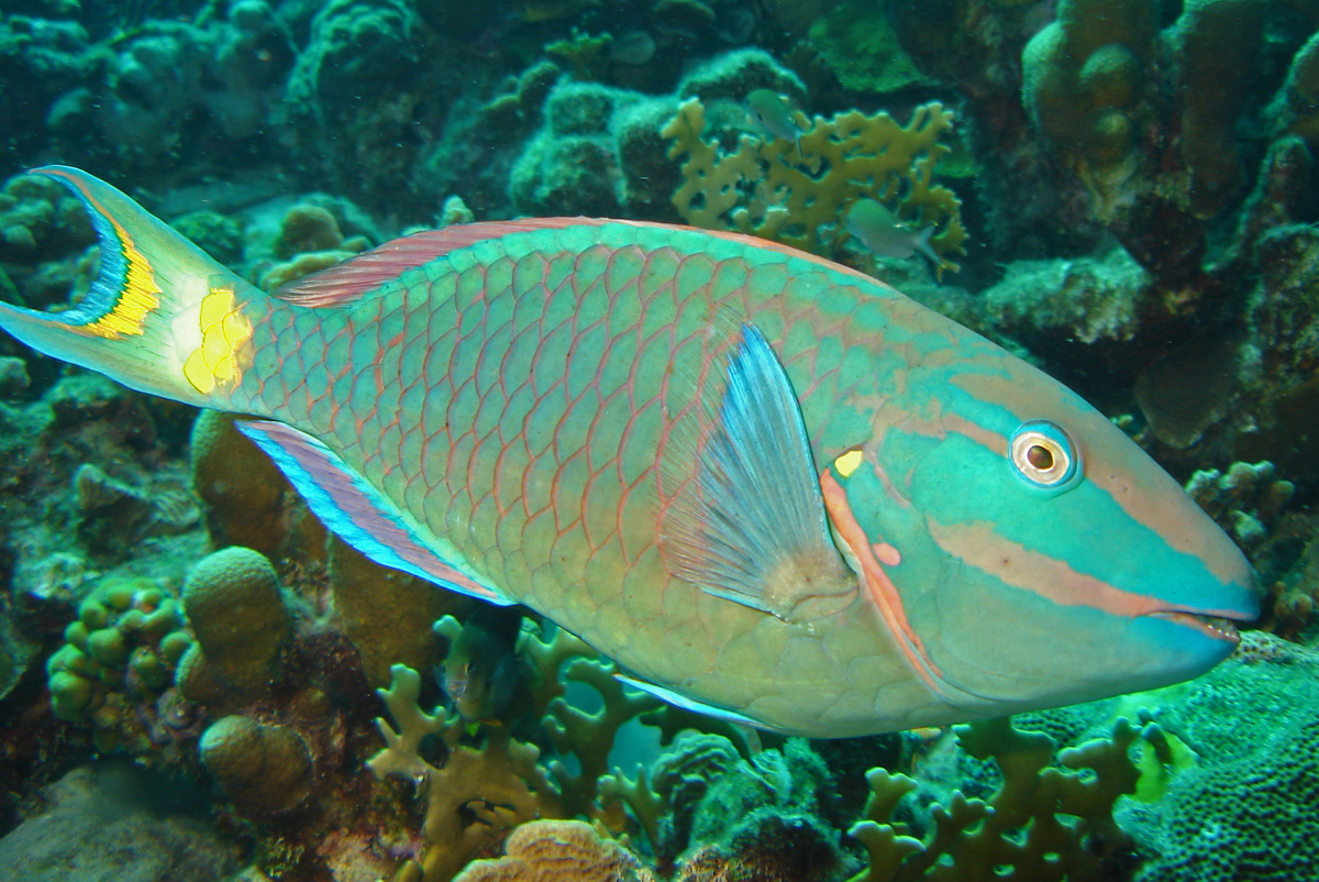
Parrotfish (over 20 cm)Stoplight parrotfish (Sparisoma viride), terminal-phase male. Parrotfish have teeth fused into a beak and large scales; bright terminal-phase males and duller initial-phase fish can look like different species. Surveys count only fish longer than 20 cm.Credit: Adona9 at English Wikipedia, CC BY-SA 3.0, via Wikimedia Commons · source 
Pencil urchinSlate-pencil urchin (Eucidaris tribuloides), Atlantic. Few, thick, blunt spines that are often coated with algae and sponges.Credit: Nhobgood (talk) Nick Hobgood, CC BY-SA 3.0, via Wikimedia Commons · source 
Pencil urchin (Indo-Pacific)Red slate pencil urchin (*Heterocentrotus mamillatus*), Indo-Pacific. Its spines are even larger and blunter than those of Eucidaris.Credit: Scott Roy Atwood, CC BY-SA 3.0, via Wikimedia Commons · source 
SnapperSchoolmaster snappers (Lutjanus apodus). Snappers have a long body, a sloping triangular head, large canine teeth and a slightly forked tail. They school by day and hunt at night.Credit: Jstuby, CC0, via Wikimedia Commons · source 
Demosponge (vase)Branching vase sponge (Callyspongia vaginalis). Sponges stay fixed in one place and pump water in through tiny pores and out through large openings (oscula).Credit: Nhobgood (talk) Nick Hobgood, CC BY-SA 3.0, via Wikimedia Commons · source 
Demosponge (barrel)Giant barrel sponge (Xestospongia muta), which can grow taller than a diver and live for centuries.Credit: Pauline Walsh Jacobson, CC BY 4.0, via Wikimedia Commons · source 
SweetlipsHarlequin sweetlips (Plectorhinchus chaetodonoides), adults. Sweetlips have thick, fleshy lips and rest in groups under ledges by day.Credit: Jens Petersen, CC BY 2.5, via Wikimedia Commons · source 
Sweetlips relative (grunt)Spanish grunt (Haemulon macrostomum). Sweetlips belong to the grunt family Haemulidae; Atlantic reefs have grunts instead of sweetlips.Credit: Jstuby, CC0, via Wikimedia Commons · source 
TritonTriton's trumpet (Charonia tritonis). A large spiral shell (up to about 50 cm) with a brown-and-cream crescent pattern. It eats sea stars, including crown-of-thorns, so collecting it for curios removes a predator.Credit: David Burdick, NOAA, Public domain, via Wikimedia Commons · source 
Fleshy algaeDictyota, a brown (Phaeophyta) fleshy alga. Fleshy algae are soft seaweeds, not hard crusts, and they spread over a reef when nutrients rise or grazers disappear.Credit: Bernard Picton, CC BY 4.0, via Wikimedia Commons · source
Indo-Pacific only

Barramundi codAlso called humpback or panther grouper (Cromileptes altivelis). A pale body with widely spaced round black spots, a small head and a concave forehead profile.Credit: Rickard Zerpe, CC BY 2.0, via Wikimedia Commons · source 
Bumphead parrotfishBolbometopon muricatum, the largest parrotfish (over 1 m). A bulbous forehead, exposed beak and green-gray color. It bites live coral and crushes it into sand.Credit: Rickard Zerpe, CC BY 2.0, via Wikimedia Commons · source 
Giant clamGiant clam (Tridacna gigas), the largest species. The wavy shell opens upward to expose a colorful mantle full of zooxanthellae.Credit: Charles J. Sharp, CC BY-SA 4.0, via Wikimedia Commons · source 
Giant clam (maxima)Maxima clam (Tridacna maxima), a smaller giant clam that bores into coral. Mantle colors vary.Credit: Alexander Vasenin, CC BY-SA 3.0, via Wikimedia Commons · source 
Humphead wrasseAlso called Napoleon wrasse (Cheilinus undulatus). A very large wrasse with thick lips, a forehead hump in big adults, and wavy lines on the face and body.Credit: Diego Delso, CC BY-SA 4.0, via Wikimedia Commons · source 
Sea cucumber (pineapple)Pineapple sea cucumber (Thelenota ananas). A large, soft, cylindrical body covered in star-shaped bumps (papillae).Credit: Diego Delso, CC BY-SA 4.0, via Wikimedia Commons · source 
Sea cucumber (greenfish)Greenfish (Stichopus chloronotus). A dark green, square-sided body with rows of pointed papillae.Credit: Paul Asman and Jill Lenoble, CC BY 2.0, via Wikimedia Commons · source
Atlantic only

Gorgonia (sea fan)Common sea fan (Gorgonia ventalina). A flat, lacy, flexible fan held across the current so its 8-tentacled polyps can catch plankton.Credit: Pauline Walsh Jacobson, CC BY 4.0, via Wikimedia Commons · source 
Flamingo tongue snailFlamingo tongue (Cyphoma gibbosum). The spotted pattern is the living mantle draped over the shell; the empty shell is plain cream-orange. It lives and feeds on gorgonians.Credit: Pauline Walsh Jacobson, CC BY 4.0, via Wikimedia Commons · source 
Nassau grouperEpinephelus striatus. Dark vertical bars, a dark "tuning-fork" mark on the forehead, a dark stripe through the eye and a black saddle spot on top of the tail base.Credit: OAR/National Undersea Research Program, Public domain, via Wikimedia Commons · source
Look-alikes and confusable pairs
Picture questions often pair an organism with a look-alike. Use this table to find the one feature that separates them.
| Confusable pair or set | Decisive feature |
|---|---|
| Long-spined black sea urchin vs pencil urchin | Diadema: many long, thin, needle-like black spines. Pencil urchin: few thick, blunt spines, often fouled with algae or sponges |
| Long-spined urchin vs crown-of-thorns starfish | Urchin: round body, spines all over, no arms. COTS: flat sea star with many arms (7–23) |
| Grouper vs Nassau grouper vs barramundi cod | All are Serranidae. Nassau: vertical brown bars, dark tuning-fork mark on the forehead and black saddle on the tail base; Atlantic. Barramundi cod: pale body with round black polka dots, small head, humped back; Indo-Pacific. Other groupers: big mouth and heavy body, many patterns |
| Parrotfish vs bumphead parrotfish vs humphead wrasse | Parrotfish: beak of fused teeth, large scales, usually under 50 cm. Bumphead parrotfish: giant parrotfish with a bulging forehead and an exposed beak, green-gray, in schools. Humphead wrasse: forehead hump too, but thick lips instead of a beak and wavy lines around the eye |
| Butterflyfish vs angelfish | Both disc-shaped and colorful. Angelfish (Pomacanthidae, not on the list) have a strong spine at the lower corner of the gill cover and are usually larger; butterflyfish lack the spine and often have an eye bar |
| Sweetlips vs grunts vs snapper | Sweetlips (Indo-Pacific) and grunts (Atlantic) share the family Haemulidae: thick lips, small mouth, no big canines. Snapper: sloping head and visible canine teeth |
| Spiny lobster vs clawed lobster vs banded coral shrimp | Spiny lobster (Palinuridae): no big claws, long thick antennae. Clawed lobster (Nephropidae): large front claws. Banded coral shrimp: small, red-white bands, long white antennae and a slender banded claw pair |
| Gorgonian vs hard coral vs sponge | Gorgonian sea fan: flexible, flat lacework, polyps with 8 feathery tentacles. Hard coral: rigid stone with cups. Sponge: no polyps or tentacles; pores and oscula, soft or rubbery |
| Triton vs flamingo tongue | Triton: huge (to about 50 cm) spindle-shaped shell with a crescent pattern, on reef or sand. Flamingo tongue: small (about 3 cm), smooth, covered by an orange-spotted mantle, always on a gorgonian |
| Sea cucumber species | Thelenota ananas: orange-red with star-shaped papillae. Stichopus chloronotus: dark green, square-sided with rows of pointed papillae |
| Giant clam vs other bivalves | Giant clam: shell sits hinge-down with a colorful mantle spread in the light; huge and wavy-edged |
| Hard coral vs bleached coral vs recently killed coral | Live coral: brown/green tissue. Bleached: white but with living, transparent tissue (counted as HC). Recently killed: bare white skeleton, often with a light film of algae (RKC) |
| Fleshy algae vs coralline algae vs turf | Fleshy algae: soft, upright seaweed. Crustose coralline algae: hard pink crusts that cement the reef (a good sign). Turf: very short algal fuzz (Reef Check records it with the substrate below) |
The salinometer task
Part IV is worth 10%: 5% just for bringing a salinometer, and 5% for an accurate reading.
Device rules
| Rule | 2027 requirement |
|---|---|
| Builder | Built, calibrated, brought and demonstrated by the team |
| Range | Salt water (most likely NaCl) from 1% to 10% mass/volume |
| Type | Salinometer or hydrometer; a simple electronic salinometer is allowed |
| Banned | Programmable devices, anything that can communicate over WiFi, laptops, tablets and similar |
| Size | No limit, but it must work in a standard 400–600 mL beaker holding at least 400 mL |
| Reading | Percent salinity to the nearest 0.1% |
| Full credit | Within ±1% at Regionals; within ±0.5% at State and Nationals |
| Calibration solutions | May or may not be supplied, so calibrate before you arrive |
Mass/volume percent means grams of salt per 100 mL of finished solution. A 3.5% m/v solution has 3.5 g of NaCl in every 100 mL.
Two designs
A hydrometer is a weighted, sealed float. By Archimedes' principle it sinks until it displaces its own weight of liquid, so in denser salt water it rides higher. Mark a scale on its stem and calibrate it. Density rises roughly in step with salinity: about 1.00 g/mL for fresh water at 20 °C, about 1.005 for 1% NaCl, about 1.025 near seawater salinity and about 1.07 near 10% (approximate; values depend on temperature). That is a total change of only about 7% across the whole range, so a thin stem gives the biggest movement per percent salt.
Both designs work for the same reason: the density and the conductivity of salt water change in a predictable, repeatable way with concentration, so a device read against known standards can be inverted to give an unknown.
An electronic (conductivity) salinometer passes a small current between two electrodes. More dissolved ions → higher conductivity → more current. A battery, two stainless or graphite electrodes at a fixed spacing and an analog meter or a calibrated LED/resistor circuit meets the "simple, not programmable" condition. Conductivity rises with temperature (roughly 2% per °C), so calibrate and test at similar temperatures.
NaCl solution density for calibration
Use this table to predict where a hydrometer should float at each standard, or to convert a measured density into a salt percentage. Values are for sodium chloride solutions at 20 °C; % m/v is found by multiplying % m/m by the density.
| NaCl (% m/m) | Density (g/mL) | NaCl (% m/v) |
|---|---|---|
| 0 | 0.998 | 0 |
| 1 | 1.005 | 1.01 |
| 2 | 1.013 | 2.03 |
| 4 | 1.027 | 4.11 |
| 6 | 1.041 | 6.25 |
| 8 | 1.056 | 8.45 |
| 10 | 1.071 | 10.7 |
Calibrating with mass/volume standards
Because the range is in m/v, make standards by dissolving a weighed mass of salt and topping up to a known final volume.
Use at least five standards across 1–10% (for example 1, 3, 5, 7 and 10%). Plot reading against known salinity and draw the best-fit line or curve; a hydrometer is close to linear, while a conductivity cell bends at high concentration. Read unknowns off the curve, not a two-point line.
Percent, ppt and specific gravity
Tests mix three ways of stating how salty water is, so be fluent in all of them.
- Percent mass/volume (% m/v): grams of salt per 100 mL of solution. 32 g of salt in 200 mL of solution is 32 ÷ 200 × 100 = 16% m/v.
- Percent mass/mass (% m/m): grams of salt per 100 g of solution. 10 g of salt + 90 g of water = 10 g in 100 g = 10% m/m. Because salt water is denser than 1 g/mL, the same solution is a little higher in % m/v than in % m/m.
- Parts per thousand (ppt, ‰) and practical salinity units (PSU): grams per kilogram of seawater. 35 ppt = 3.5%. PSU is a unitless scale based on conductivity; numerically it is almost the same as ppt.
- Specific gravity: density of the sample ÷ density of pure water at the same temperature. A hydrometer reads it directly. Seawater is about 1.025.
| Water type (simple scheme) | Salinity (ppt) | Example |
|---|---|---|
| Fresh | < 0.5 | Rivers, most lakes |
| Brackish | 0.5–30 | Estuaries, mangrove creeks |
| Saline (seawater) | 30–50 | Open ocean, about 35 |
| Brine (hypersaline) | > 50 | Salt ponds, desalination reject water, Dead Sea |
This simple four-way scheme is common on tests; the more detailed Venice system (in Salinity classes) splits brackish water into oligo-, meso- and polyhaline and calls 30–40 ppt euhaline. Use the scheme the question names.
A straw salinometer is the simplest hydrometer: a drinking straw weighted at one end (clay, a pin or a BB) and sealed, floated upright, with marks for known salinities. It works by buoyancy.
Sources of error and which way they push the reading
Questions ask which way an error pushes the reading, and you need the same reasoning to debug your own device. Work each case in two steps: what happens physically, then what the scale reports.
| What happened | Hydrometer (density) device | Conductivity device |
|---|---|---|
| Test water warmer than calibration water | Warm water is less dense → device sinks deeper → reads low (underestimates) | Ions move faster → conductivity rises about 2% per °C → reads high (overestimates) |
| Test water colder than calibration water | Denser → floats higher → reads high | Conductivity falls → reads low |
| Float absorbs water or a leak lets water in | Heavier → sinks deeper → reads low | — |
| Air bubble clinging to the float | Extra buoyancy → floats higher → reads high | Bubble on an electrode cuts current → reads low |
| Salt crust left on the device | Heavier → reads low | Residue dissolves into the sample → reads high |
| Unknown is not NaCl (e.g. contains KCl) | Responds to density of whatever salt is present | KCl conducts differently per gram than NaCl, so a mixed unknown reads wrong in a direction that depends on the salt; calibrate with the same salt you will be tested with |
| Electrodes deeper or closer than during calibration | — | More electrode area or a shorter gap → more current → reads high |
Getting the reading right
- Rinse the device with distilled water and blot it between samples so you do not carry salt across.
- Read a hydrometer at eye level at the bottom of the meniscus; tap it to release air bubbles.
- Let a conductivity cell settle and keep the electrodes at the same depth every time.
- Measure the sample temperature and compare with your calibration temperature.
- Practice the full routine with unknowns made by a teammate until you are inside ±0.5% every time.
- Bring Category C goggles, or you cannot test.
Glossary and quick facts
Tests in this event reward vocabulary. Many questions are a single term, a definition, a "which is NOT" list or a one-line fact. This chapter collects the terms, numbers and list-style answers that come up on real tests but are not taught elsewhere in the guide. The main chapters still hold the core ideas: when a term here builds on one of them, the row points you to that section.
How to use it:
- Look up an unfamiliar term with the filter box on each table. The terms are grouped by theme, so related words sit next to each other. Read the neighbors too, because tests like to offer a related term as a distractor.
- Skim the quick-facts table the week before a tournament. Each row is one number or named example that a question has asked for.
- Practice the short-answer patterns by covering the bullets and listing them from memory. Most free-response questions on past tests ask you to "list" or "name" three or four items, and each correct item earns a fraction of a point.
Glossary of chemistry and monitoring terms
These are physical-chemistry words, instrument names and measurement terms. For the 11 parameters themselves, see The 11 parameters at a glance.
ReferenceGlossary: chemistry and monitoring terms· 34 rows
Terms are roughly grouped: water's physical behavior, carbonate minerals and scaling, measurement units and instruments, then dissolved organic matter and microbes.
No rows match.
| Term | Meaning | Example or why it matters |
|---|---|---|
| Density anomaly (anomalous expansion of water) | Liquid fresh water gets denser as it cools only down to about 4 °C. Below that it expands again, and ice is about 8–9% less dense than liquid water (0.917 vs about 1.000 g/cm³) | This is why ice floats, why it insulates a lake from above, and why the bottom of an ice-covered lake stays near 4 °C |
| Viscosity | A fluid's internal resistance to flow (its "thickness") | Water's viscosity roughly halves between 0 °C and 25 °C. Particles and plankton therefore sink faster in warm water, which is one reason warm-water plankton carry extra spines and flattened shapes |
| Reynolds number (Re) | A dimensionless ratio of inertial forces to viscous forces in a flow. Low Re gives smooth, layered (laminar) flow, and high Re gives turbulent flow | In pipes, flow is usually laminar below about 2,000 and turbulent above about 4,000. Plankton live at very low Re, so to them water behaves like syrup |
| Brownian motion | Random jiggling of tiny suspended particles, caused by uneven bombardment from moving water molecules | Together with the like electric charges that make colloids repel each other, it keeps them from settling on their own, which is why coagulation is needed in water treatment |
| True solution, colloid, suspension | Classes of particle size. Dissolved molecules and ions are below about 1 nm and never settle. Colloids are about 1 nm to 1 µm, stay suspended and scatter light. Suspended particles are larger than about 1 µm and settle when the water stands still | Coagulation and flocculation target the colloids. Plain sedimentation removes the larger suspended particles. The boundaries are approximate |
| Tyndall effect | A beam of light becomes visible because colloidal particles scatter it | This scattering is the physical basis of nephelometric (90°) turbidity meters |
| Amphiphilic (amphipathic) | Describes a molecule with one water-loving (polar) part and one water-fearing (nonpolar) part | Soaps, detergents, oil dispersants and many protein-denaturing chemicals are amphiphilic. They collect at oil–water boundaries |
| Surfactant | An amphiphilic compound that lowers surface tension | Surfactants are found in detergents in wastewater. Oil dispersants are surfactants that break slicks into droplets |
| "Potential of hydrogen" (also "power of hydrogen") | The usual expansion of the abbreviation pH. In practice pH = −log[H⁺], and [H⁺] means the same as [H₃O⁺] | See pH and aragonite saturation for the calculations |
| Aragonite | An orthorhombic crystal form of CaCO₃. It is denser and more soluble than calcite | Stony corals, pteropods and many larval shells are made of aragonite, so these organisms feel ocean acidification first |
| Calcite | A trigonal (rhombohedral) crystal form of CaCO₃. It is the more stable and less soluble form | Coccolithophores, foraminifera and many adult mollusk shells are made of calcite. Limestone is mostly calcite |
| High-magnesium calcite | Calcite with a few percent or more (often above about 4 mol%) of Mg in place of Ca. Above roughly 12 mol% MgCO₃ (typical of coralline algae) it is more soluble than aragonite | It is made by crustose coralline algae and sea urchins, so coralline algae are especially sensitive to acidification |
| Orthorhombic | A crystal system with three unequal axes, all at right angles to each other | This is the answer to "what crystal system is aragonite?" |
| Calgon | A trade name for sodium hexametaphosphate, a sequestering (chelating) agent that holds Ca²⁺ and Mg²⁺ in soluble complexes | It is classically listed as a treatment for permanent (non-carbonate) hardness, which boiling cannot remove |
| Sequestering (chelating) agent | A chemical that binds metal ions into a stable, soluble complex so they cannot react | Examples are EDTA (used in the hardness titration) and polyphosphates (used to stop scale and iron staining) |
| Langelier saturation index (LSI) | LSI = actual pH − pHₛ, where pHₛ is the pH at which the water would be exactly saturated with CaCO₃. A positive LSI means the water tends to deposit scale, and a negative LSI means it is corrosive | This is the plumbing version of the saturation idea behind aragonite Ω. A water that is undersaturated in CaCO₃ dissolves carbonate |
| Ryznar and Puckorius indexes | Scaling indexes built on the same pHₛ idea (Ryznar = 2pHₛ − pH; Puckorius uses an "equilibrium pH" set by alkalinity). Low values (below about 6) mean scaling and high values (above about 7) mean corrosion | They are used for cooling water, aquaculture and aquarium systems. Know that they predict scale versus corrosion, not salinity |
| Cathodic protection | Stopping metal corrosion by making the structure the cathode of a cell. This is done with sacrificial anodes (zinc, aluminum, magnesium) or with an impressed electric current | Ship hulls, piers, offshore platforms and pipelines use it. It is checked by measuring the structure's potential against a reference electrode |
| Silver/silver chloride (Ag/AgCl) reference electrode | A stable reference electrode made of silver coated with AgCl | It is the standard reference for corrosion checks in seawater. Copper/copper-sulfate electrodes are used in soil. An Ag/AgCl reference is also inside most combination pH electrodes |
| FTU (formazin turbidity unit) | A turbidity unit based on a formazin polymer standard, without specifying the instrument geometry | The related units are NTU (white light, 90° detector), FNU (infrared light, 90°) and JTU (Jackson candle). They are roughly equal for formazin standards |
| Isopleth | A line on a map or cross-section joining points of equal value | The named types are isohaline (salinity), isotherm (temperature), isopycnal (density), isobath (depth) and isobar (pressure) |
| Bathymetry | The measurement and mapping of water depth and seafloor shape, mostly by echo sounding (sonar, including multibeam) | Bathymetric charts show isobaths. Seafloor shape steers currents and upwelling |
| Spectrophotometer | An instrument that measures how much light of a chosen wavelength a colored sample absorbs | It is used for nitrate (cadmium reduction or similar), phosphate (molybdenum blue) and ammonia. See Colorimetry and Beer's law |
| Atomic absorption spectroscopy (AAS) | Atomizes the sample in a flame or graphite furnace and measures the light absorbed at each metal's own wavelength | Measures individual heavy metals (lead, cadmium, copper, zinc) at µg/L levels |
| ICP-OES / ICP-MS | Inductively coupled plasma: a very hot argon plasma atomizes the sample, then either the emitted light (OES) or the ion masses (MS) are measured | Measures many metals at once. ICP-MS reaches trace (ng/L) levels |
| Atomic fluorescence spectroscopy (AFS) | Measures the light re-emitted by excited atoms | Especially sensitive for mercury, arsenic and selenium |
| Gas chromatography–mass spectrometry (GC-MS) | Separates volatile organic compounds in a column (GC), then identifies each one by its mass fragments (MS) | This is the standard method for pesticides, PCBs, PAHs and other organic pollutants. LC-MS handles compounds that do not vaporize well |
| Ion chromatography | Separates dissolved ions on an exchange column and detects them, usually by conductivity | Measures nitrate, nitrite, phosphate, sulfate, chloride and fluoride in one run |
| Fluorometer | Excites a sample with one wavelength of light and measures the light given off at a longer wavelength | Measures chlorophyll a in the field or on sondes, and also tracer dyes and some oils |
| Dissolved organic carbon (DOC) | Organic carbon that passes through a fine filter. The cutoff is set by the method: usually 0.45 µm, or 0.7 µm glass-fiber filters in oceanography, sometimes 0.2 µm. What the filter keeps is particulate organic carbon (POC) | DOC absorbs UV and blue light, so it shields microbes from UV disinfection. It also reacts with chlorine to form disinfection byproducts |
| CDOM (colored dissolved organic matter) | The part of dissolved organic matter that absorbs light, mostly humic substances. It tints water yellow-brown (the old name is gelbstoff, "yellow substance") | It is high in estuaries and blackwater rivers. It reduces light for seagrass and confuses satellite chlorophyll estimates |
| Psychrophile, mesophile, thermophile, hyperthermophile | Microbes with optimum growth temperatures of roughly below 15 °C, 20–45 °C, 45–80 °C, and above 80 °C respectively | Hyperthermophilic archaea live at hydrothermal vents. Most fecal and wastewater bacteria are mesophiles |
| Enterobacteriaceae | A family of Gram-negative, rod-shaped, non-spore-forming, facultatively anaerobic bacteria that includes E. coli, Salmonella, Shigella, Klebsiella and Enterobacter | Coliforms are a lactose-fermenting group drawn mostly from this family. Ones that ferment lactose at 44.5 °C are thermotolerant (fecal) coliforms |
| TNTC / TFTC | "Too numerous to count" and "too few to count" on a membrane-filtration or pour plate | Standard Methods gives an ideal count of about 20–80 coliform colonies per 47 mm membrane (20–60 for fecal coliform), with no more than about 200 colonies of all types. Outside that range, redo the test with a different sample volume |
The two easiest confusions in this table are aragonite versus calcite (aragonite is the more soluble one and the one corals use) and FTU versus FNU (both use formazin standards; FNU also specifies an infrared, 90° instrument).
Glossary of ecology and oceanography terms
These terms cover energy flow, life history, wetlands, coastal landforms and the physics of moving water. For the core ideas, see Marine and estuary ecology.
ReferenceGlossary: ecology and oceanography terms· 62 rows
Terms are grouped: energy and food webs, adaptations and evolution, wetlands, coasts and lakes, then water and air movement.
No rows match.
| Term | Meaning | Example or why it matters |
|---|---|---|
| Allochthonous | Organic matter or energy that comes from outside the water body | Leaves and woody debris falling into a stream, or marsh detritus washed into a bay. Shaded headwater streams and many estuaries run largely on allochthonous carbon |
| Autochthonous | Organic matter produced inside the water body by its own algae, phytoplankton and aquatic plants | Open-ocean food webs and large sunny lakes run mainly on autochthonous production |
| Consumption efficiency | The percentage of the production at one trophic level that the next level actually eats | Low when much plant matter goes uneaten to decomposers, as in marshes. Higher in phytoplankton systems, where grazers eat most cells |
| Assimilation efficiency | The percentage of eaten food that is absorbed rather than egested | Carnivores (about 80%) absorb more of their food than herbivores eating tough plants (about 20–50%). These are textbook approximations |
| Production efficiency | The percentage of assimilated energy that becomes new biomass (growth and reproduction) rather than being respired | Ectotherms (fish, invertebrates) score much higher than birds and mammals, which burn energy to stay warm |
| Trophic (ecological) efficiency | Consumption × assimilation × production efficiency: the share of one level's production that becomes production at the next level | About 10% on average, which is the basis of the 10% rule |
| Predator–prey mass ratio (PPMR) | The average body mass of a predator divided by the mass of its prey | A larger PPMR means each step covers a bigger jump in size, so fewer steps separate tiny producers from top predators and the food chain is shorter. A smaller PPMR means a longer chain |
| Island biogeography | The theory (MacArthur and Wilson) that the number of species on an "island" is a balance between colonization and extinction | Larger islands (or lakes and reefs) have lower extinction rates. Islands closer to a source have higher colonization rates. The theory applies to isolated lakes, reefs and marine reserves |
| Directional selection | Selection that favors one extreme of a trait, so the population average shifts | Guppies in streams with more predators evolve duller colors. Fishing that removes the biggest fish selects for smaller, earlier-maturing fish |
| Stabilizing selection | Selection that favors the average and removes both extremes | Fish eggs of intermediate size often survive best |
| Disruptive selection | Selection that favors both extremes over the average, which can split a population | Seen in some fish with two feeding types, such as cichlids with two distinct jaw morphs (crushing versus slender jaws for different foods) |
| Foraging strategy | How an animal finds and handles food: ambush (sit-and-wait), active pursuit, grazing, filter feeding, scavenging | Ambush examples are the frogfish and lionfish. Groupers also mostly lie in wait. Jacks and tuna pursue prey, parrotfish graze, and giant clams and sponges filter feed |
| Poikilotherm (ectotherm) | An animal whose body temperature follows that of its surroundings and depends on outside heat | Most fish and invertebrates. When water warms, their metabolism and oxygen demand rise just as DO falls |
| Homeotherm (endotherm) | An animal that holds a steady internal temperature by making its own heat | Marine mammals and seabirds rely on blubber, feathers and countercurrent heat exchangers |
| Countercurrent exchange | Two fluids flow in opposite directions past each other, so a diffusion gradient is kept along the whole length of the exchanger | In fish gills, water and blood flow in opposite directions, letting fish extract a large share (commonly cited around 80%) of the oxygen in the water. The same arrangement conserves heat in whale flippers and tuna muscle |
| Bycatch | Animals caught unintentionally in fishing gear, or caught but unwanted, and often thrown back dead or dying | Sea turtles in shrimp trawls (turtle excluder devices reduce this), and dolphins and sharks on longlines |
| Mycoplankton | Fungi (and fungus-like organisms) living in the plankton | They are decomposers and parasites of phytoplankton. Do not confuse them with bacterioplankton |
| Periphyton | The mixed film of algae, bacteria, fungi and detritus attached to submerged surfaces such as rocks, plants and pilings. It is also called aufwuchs or biofilm | It is food for grazing snails and other scrapers. Its growth is an early sign of nutrient enrichment |
| Functional feeding groups | A way of classifying benthic invertebrates by how they feed: shredders (chew coarse leaf litter), collectors (gather or filter fine particles), scrapers or grazers (scrape periphyton and biofilm off surfaces) and predators | In the river-continuum idea, shredders dominate shaded upper reaches. Scrapers increase where light reaches the bed. These groups are used in stream biomonitoring |
| Wetland | Land that is flooded or saturated long enough, often seasonally, to have hydric soils and hydrophytes (plants adapted to saturated soil). Water comes mainly from surface water and groundwater, plus precipitation and tides | The three delineation criteria are hydrology, hydric soils and hydrophytic vegetation. Seasonal soil saturation, not permanent open water, separates a wetland from a lake |
| Hydric soil | Soil formed under saturation long enough to become anaerobic. It shows gray colors, mottles or a sulfur smell | Used as evidence of a wetland even when the site is dry |
| Halophyte | A plant that tolerates salty soil or water | Smooth cordgrass (Spartina alterniflora), glassworts (Salicornia) and mangroves |
| Wetland indicator status | U.S. categories for how often a plant occurs in wetlands (older numeric definitions; the current list uses descriptive ones). OBL (obligate): more than 99% of the time. FACW: 67–99%. FAC: 34–66%. FACU: 1–33%. UPL: less than 1% | Obligate wetland plants include cattails, duckweed, water lilies, pickerelweed and smooth cordgrass |
| Cowardin systems | The U.S. Fish and Wildlife Service wetland classification: Marine, Estuarine, Riverine, Lacustrine (lakes) and Palustrine | Estuarine wetlands are tidal and brackish. Marine wetlands are open-coast intertidal areas |
| Palustrine | Non-tidal vegetated wetlands (marshes, swamps, bogs, fens, wet meadows), plus small ponds under 8 ha. Tidal areas belong here only if salinity is below 0.5 ppt | Most inland freshwater marshes, swamps and bogs are palustrine |
| Marsh | A wetland dominated by soft-stemmed herbaceous plants (grasses, rushes, cattails) | Salt marsh, brackish marsh and tidal freshwater marsh |
| Swamp | A wetland dominated by trees or shrubs | Cypress swamps, and mangrove swamps on tropical coasts |
| Bog | An acidic, nutrient-poor peat wetland fed mainly by rain | Sphagnum moss, carnivorous plants, tea-colored water |
| Fen | A peat wetland fed by groundwater, so it is less acidic and richer in minerals than a bog | Sedges and grasses dominate |
| Pocosin | An evergreen shrub bog on deep, acidic, nutrient-poor peat on the Southeastern U.S. Coastal Plain, especially North Carolina | It is a type of palustrine wetland. The name comes from an Algonquian word often translated "swamp on a hill" |
| Vernal pool | A temporary, shallow pool that fills in winter or spring and dries by summer | It has no fish, so it is a key breeding site for amphibians and fairy shrimp |
| Mangal | The scientific term for a mangrove forest community (the mangrove biome) | See Mangrove forests |
| Thalassic | Saline water of marine origin: seawater and its mixtures with fresh water. The Venice-system classes (oligohaline to hyperhaline) form the thalassic series | Estuaries and coastal lagoons are thalassic |
| Athalassic | Inland saline water whose salts did not come from the sea, so the ion ratios differ from seawater | The Great Salt Lake, the Dead Sea and soda lakes |
| Infralittoral zone | The shallow subtidal zone from the low-tide mark down to the depth where algae stop dominating | It is the algae-dominated zone (kelp and seaweed beds). The circalittoral below it is dominated by animals (sponges, sea fans, bryozoans) |
| Eulittoral (midlittoral) zone | The main intertidal zone between high- and low-tide marks | Barnacles, mussels and limpets show clear vertical bands here |
| Spray zone (splash zone, supralittoral) | The zone above high tide that is wetted only by spray and storm waves | Periwinkles and lichens live here. It has the most extreme temperature and drying stress |
| Subtidal benthos | Bottom-dwelling organisms below the low-tide line | They have the most stable temperature of all shore habitats, because they are never exposed to air |
| Barrier beach | A long, narrow ridge of sand parallel to the shore, shaped by strong waves, wind and shifting sand. It is called a barrier island if separated from the mainland and a spit if one end is attached | Barrier beaches enclose lagoons and bar-built estuaries such as the Outer Banks |
| Tombolo | A sand bar that connects an island to the mainland | A depositional landform, often given as a distractor in estuary questions |
| Marine terrace | A flat, step-like platform that marks a former shoreline cut by waves | Most are raised above sea level by uplift (as on the California coast). A submerged coast shows drowned river valleys (estuaries) instead |
| Glacial flour (rock flour) | Silt- and clay-sized rock powder ground by glaciers | It makes meltwater rivers and lakes milky and turquoise: high turbidity from a natural source |
| Dystrophic lake | A brown, humic-stained, usually acidic lake with low productivity, typical of bogs and peatlands | It usually has the lowest species richness of the lake trophic types. See Trophic states |
| Oligotrophication | A decline in nutrient supply and therefore in productivity: the reverse of eutrophication | This happens after strict phosphorus controls, or when invasive mussels filter out plankton (Lake Huron is an example) |
| Dimictic, monomictic, meromictic | Dimictic lakes turn over twice a year (spring and fall; typical temperate lakes). Monomictic lakes turn over once (warm lakes in winter, or cold lakes in summer). Meromictic lakes never mix fully, because a dense, salty or anoxic bottom layer stays isolated | Amictic lakes (never mix, ice-covered) are covered in Lake zones, for comparison |
| Overturn (turnover) cause | Turnover happens when the surface water reaches the same density as the bottom water, so the stratification is no longer stable and wind can mix the whole lake. In fall the surface cools to about 4 °C. In spring the ice melts and the surface warms to about 4 °C | Turnover gives uniform temperature and DO top to bottom, and it carries nutrients up and oxygen down |
| Winterkill | A fish die-off under ice and snow cover: light is blocked, photosynthesis stops, and decomposition uses up the dissolved oxygen | It is most likely in shallow, eutrophic lakes. Summerkill is the warm-season version, from hot weather, algal die-offs and stratification |
| Groundwater recharge zone | An area where water infiltrates and moves down to the water table | Paving recharge zones reduces aquifer supply |
| Groundwater discharge zone | An area where groundwater flows out into a stream, lake, spring, wetland or estuary | Gaining streams receive groundwater. Losing streams leak water into the ground |
| Porosity | The fraction of a rock or soil's volume that is open pore space | Clay has high porosity but low permeability |
| Permeability | How easily water moves through connected pores and fractures | Topsoil permeability and rock porosity control recharge and spring flow in karst |
| Soil texture | The proportions of sand (0.05–2 mm), silt (0.002–0.05 mm) and clay (below 0.002 mm), using USDA sizes | Sandy soils drain fast and filter poorly. Clay soils drain slowly and erode into long-lasting turbidity |
| Loam | Soil with roughly balanced amounts of sand, silt and clay | It drains well while holding moisture and nutrients. It is the ideal farm soil |
| Sinuosity | The channel length of a stream divided by the straight-line valley length. Above about 1.5 the stream is called meandering | Extra sediment load pushes a river out of equilibrium, changing sinuosity, bars and channel shape |
| Channelization | Straightening, deepening or lining a stream channel | Water moves faster, banks and beds erode, turbidity rises, flooding moves downstream and habitat is lost |
| Eddy | A rotating swirl of water that has broken off a current. Ocean eddies are often 10–200 km across. Warm-core and cold-core rings shed by the Gulf Stream are examples | Eddies carry heat, nutrients, larvae, plankton and pathogens long distances |
| Ocean front | A sharp boundary between two water masses with different temperature or salinity | Plankton, debris and predators gather along fronts. Persistent fronts can carry organisms long distances |
| Internal waves and internal tides | Waves that travel along a density boundary (the pycnocline) beneath the surface. Internal tides are internal waves with tidal periods | They can be tens of meters high. They mix nutrients up onto reefs and shelves, and they move larvae and pathogens |
| Cascading (dense shelf-water cascading) | Shelf water that becomes colder or saltier than offshore water at the same depth (from winter cooling, evaporation or ice formation) flows down the continental slope as a dense current | It carries sediment, organic carbon and oxygen to the deep sea |
| Caballing | Two water masses of equal density but different temperature and salinity mix to form water that is denser than either, so it sinks | It happens because the density of seawater does not change linearly with temperature and salinity |
| Dry deposition | Gases and particles (nitrogen compounds, dust, mercury) settling from the air without rain. Wet deposition is the same material brought down in rain or snow | Atmospheric deposition is a source of new nitrogen for coastal waters, along with river transport and nitrogen fixation |
| Urban heat island | Cities stay warmer than the surrounding countryside, because dark pavement and buildings absorb heat and there is little vegetation or evaporation | Warm runoff from hot pavement is a form of thermal pollution in urban streams. Green roofs, trees and light-colored surfaces reduce it |
Glossary of pollution, treatment and management terms
These terms are about treatment plants, cleanup and land management. For the treatment sequences themselves, see Water treatment.
ReferenceGlossary: pollution, treatment and management terms· 33 rows
Terms are grouped: wastewater plant terms, drinking-water and membrane terms, cleanup and remediation, then land and fisheries management.
No rows match.
| Term | Meaning | Example or why it matters |
|---|---|---|
| Influent | Raw water or wastewater flowing into a treatment plant or process unit | Plant efficiency is (influent − effluent) ÷ influent × 100% |
| Effluent | Treated (or partly treated) water flowing out of a plant, unit or factory | A factory effluent pipe is the classic point source |
| Comminution | Grinding or shredding coarse solids in the incoming wastewater (with a comminutor) instead of screening them out | The shredded solids stay in the flow and are removed later in the clarifiers |
| Reserve capacity | Extra treatment and pipe capacity built into a new plant or sewer so it can handle future growth in flow | Plants are designed for the population expected decades ahead |
| Roughing filter | A high-rate trickling filter placed before the main biological treatment to cut the BOD load of strong wastewater. In drinking-water treatment, a coarse gravel filter that lowers turbidity before slow sand filtration | Answer "roughing filter" when asked which unit reduces BOD. An API oil–water separator removes free oil, not BOD |
| Biochemical oxidation | Microbes oxidizing dissolved and colloidal organic matter to CO₂, water and new cells | This is the core of secondary treatment. The organic matter is the "food supply" for the bacteria |
| Extended aeration | An activated-sludge process with a long aeration time (about a day) and old sludge, so the microbes digest much of their own biomass | It produces little sludge, is stable and simple, and suits small plants |
| Oxidation ditch | An extended-aeration process in an oval "racetrack" channel stirred by rotors or brushes | It handles shock loads and cold weather well. Aerated and low-oxygen zones in the loop let it nitrify and denitrify |
| Sulfate-reducing bacteria (SRB) | Anaerobic bacteria that use sulfate in place of oxygen, producing hydrogen sulfide | In treatment, they precipitate dissolved metals as insoluble metal sulfides and raise pH, which is useful for acid-mine and toxic metal streams. In pipes, they cause rotten-egg odor and corrosion |
| Bioconcentration | A chemical builds up in an organism directly from the water (across gills or skin), not from food. It is measured by the bioconcentration factor (BCF) = concentration in the organism ÷ concentration in the water | Bioaccumulation includes uptake from food as well. Biomagnification is the increase from one trophic level to the next |
| Biotransformation | Organisms chemically changing a substance into other compounds. It includes biodegradation | Bacteria convert inorganic mercury to methylmercury, a biotransformation that makes it far more toxic |
| Methylmercury toxicity | MeHg is absorbed readily from the gut, binds to the sulfhydryl (–SH) groups of proteins, and crosses the blood–brain barrier and the placenta | This is why it biomagnifies and damages the nervous system. Selenium can bind mercury and partly reduce its toxicity |
| Thermal enrichment | A case where heated discharge benefits some part of an ecosystem, for example longer growing seasons, or manatees and fish gathering at warm outfalls in winter | It is the positive counterpart of thermal pollution. Warmer water also makes organisms more vulnerable to disease, parasites and toxic chemicals |
| Retention pond (wet pond) | A stormwater basin that holds a permanent pool of water | Sediment settles out and plants and microbes take up nutrients, so it treats water as well as storing it |
| Detention basin (dry pond) | A stormwater basin that holds runoff temporarily and drains empty within a day or two | It mainly cuts peak flow and erosion and settles some sediment |
| Electrofishing and electric barriers | Electrofishing passes a controlled current through water to stun fish briefly for counting or removal. An electric barrier is a field across a channel that fish will not cross | The Chicago Sanitary and Ship Canal barriers are meant to keep Asian carp out of the Great Lakes |
| Bioremediation | Using organisms, mainly microbes, to break down or capture pollutants | It is slower than mechanical cleanup but cheap and low-impact. It is the last step of many oil-spill responses |
| Bioventing | Pumping air into the unsaturated soil zone to speed up microbial breakdown of contaminants in place | Used for fuel-contaminated soil above the water table |
| Biosparging | Injecting air (and sometimes nutrients) into the saturated zone below the water table | Used for contaminated groundwater |
| Bioattenuation (monitored natural attenuation) | Leaving native microbes to degrade a contaminant while monitoring that it is shrinking | Used where the risk is low |
| Biostimulation, bioaugmentation | Biostimulation adds nutrients or oxygen to boost native microbes. Bioaugmentation adds cultured microbes | Fertilizing oiled beaches after the Exxon Valdez spill was biostimulation |
| Phytoremediation | Using plants to remove, hold or break down pollutants. Hyperaccumulator plants concentrate metals in their tissues, which are then harvested | Sunflowers and Indian mustard have been used for metals, and willows and poplars for groundwater plumes |
| Landfarming | Spreading contaminated soil or sludge thinly and tilling it so that soil microbes degrade it | Used for petroleum-contaminated soil |
| Thermal desorption | Heating contaminated soil so organic pollutants evaporate and can be captured | It is a soil-cleanup method, not a desalination method. It is a common distractor |
| Natural recovery (oil spills) | Deciding not to intervene and letting evaporation, wave action and biodegradation remove the oil | Chosen for exposed, high-energy rocky shores where cleanup would do more harm than good |
| Membrane filtration ladder | From coarse to fine, by roughly the smallest particle each removes. Microfiltration (about 0.1 µm): particles, protozoa and most bacteria. Ultrafiltration (about 0.01 µm): also viruses and large organics. Nanofiltration (about 0.001 µm): hardness ions and many organics. Reverse osmosis: dissolved salts | The EPA lists microfiltration among the processes for removing suspended particles and pathogens. Only nanofiltration and RO remove dissolved ions |
| Point-of-use filter (for example, the LifeStraw) | A personal hollow-fiber membrane filter (about 0.2 µm) that strains out sediment, bacteria and protozoa | It does not remove dissolved chemicals such as heavy metals, pesticides, petroleum compounds or salt. The basic version is not rated for viruses |
| Crystallizer | The last stage of a zero-liquid-discharge system. It turns concentrated brine into solid salt. The types are forced-circulation, draft-tube-baffle and surface-cooled crystallizers | "Solidified suspensions" is not a crystallizer type |
| API oil–water separator | A gravity tank (to an American Petroleum Institute design) in which free oil floats off and solids sink | Used for refinery and industrial wastewater. It is not a BOD-removal or desalination unit |
| EDR (electrodialysis reversal) | Electrodialysis with the polarity flipped periodically to clean scale off the membranes | Used to desalt brackish water |
| Pipe color code | The "Ten States Standards" plant scheme (recommended standards used by many U.S. states): finished or potable water dark blue, raw water olive green, sludge dark brown, sewer lines dark gray, chlorine yellow, compressed air dark green, gas lines red | Local codes vary, so treat the scheme as commonly cited. In this scheme ozone lines are yellow with orange bands, not pink |
| Sarno River | A river near Naples in southern Italy, often called the most polluted river in Europe, because of untreated industrial (tannery and cannery), agricultural and sewage discharges | A named example of severe point-source and nonpoint-source pollution |
| International Whaling Commission (IWC) | The body that regulates whaling. A commercial moratorium has applied since 1986 | Japan and Norway have pushed for commercial quotas, mainly on minke whales. Norway hunts under a formal objection, and Japan left the IWC in 2019 |
The two most-swapped pairs here are retention versus detention (wet versus dry) and bioventing versus biosparging (above versus below the water table).
Glossary of reef and organism terms
Most reef vocabulary is in Coral reefs and the Indicator organism reference. This short table covers the remaining terms that past tests ask for.
ReferenceGlossary: reef and organism terms· 9 rows
No rows match.
| Term | Meaning | Example or why it matters |
|---|---|---|
| Red band disease | A coral disease in which a red-brown band of filamentous cyanobacteria moves across the colony and leaves bare skeleton behind it | Seen on Caribbean brain and star corals. It is easily confused with black band disease, which forms a darker mat |
| Coral pathogen detection | PCR detects a pathogen's DNA. Dipstick (lateral-flow) assays use antibodies for a quick field test. Fluorescence microscopy (including FISH) lights up labeled microbes in tissue. Culturing grows suspected pathogens | All of these are real tools. Disease is first spotted in the field from lesion patterns |
| Other reef builders | Besides stony (scleractinian) corals: crustose coralline algae (cement and build the reef crest); fire corals (Millepora, hydrozoans); blue coral (Heliopora) and organ-pipe coral (Tubipora), which are octocorals with hard skeletons; Halimeda (makes sand); and tube-building worms (serpulid and sabellariid reefs), vermetid snails and oysters | Coralline algae build and cement the reef. They do not break down limestone; that is bioerosion by parrotfish, urchins and boring sponges |
| Spongin | A flexible collagen-like protein forming the soft skeleton of many sponges | Bath sponges are dried spongin skeletons |
| Spicules | Tiny skeletal needles or stars of silica or calcium carbonate inside sponge tissue | Spicule shape and chemistry are used to classify sponges. Sponges also make bioactive compounds that deter predators. Only a few animals, mainly hawksbill sea turtles and some angelfish and filefish, eat them in quantity |
| Sponge reproduction | Asexual by budding, fragmentation and gemmules (resistant internal buds). Sexual by sperm released into the water, with larvae that swim | Sponges do not form spores |
| Annelida | Segmented worms (polychaetes, earthworms, leeches) with a true coelom. Many polychaetes reproduce both sexually and asexually | Christmas tree and feather duster worms are filter-feeding reef polychaetes. Bristle worms are prey for sweetlips |
| Vaucheriaxanthin | A carotenoid pigment characteristic of the yellow-green algae (Xanthophyceae, for example Vaucheria) | Algal groups are told apart by their pigments: phycoerythrin in red algae, fucoxanthin in brown algae and diatoms |
| Triton larva | A long-lived planktonic (teleplanic) veliger larva that drifts in the water column for months | This long drifting stage explains how the giant triton reaches reefs across the Indo-Pacific |
Quick facts and numbers
Each row below is a single fact or named example that tests have asked for. Facts taught in the main chapters (instruments, standards, lead, sunscreen laws) are not repeated here. "Commonly cited" marks a textbook approximation; if a test offers a range, choose the option that contains this value.
ReferenceQuick facts and numbers· 13 rows
No rows match.
| Fact | Value | Note or source type |
|---|---|---|
| Where Earth's fresh water is stored | About 69% in ice caps and glaciers, about 30% groundwater, about 1% surface and other fresh water | USGS. Lakes and rivers together hold well under 1% of fresh water |
| Saltiest marginal seas | Red Sea about 40 ppt, Mediterranean about 38–39 ppt. Both are well above the open ocean (about 35) | High evaporation, little river input and restricted exchange. Among the major oceans, the Atlantic is the saltiest on average |
| Typical tap-water pH | About 7, near neutral (U.S. secondary standard 6.5–8.5) | Utilities often raise pH slightly to limit pipe corrosion |
| Fluoride in drinking water | U.S. recommended level for preventing tooth decay is 0.7 mg/L. EPA MCL 4.0 mg/L. Secondary standard 2.0 mg/L (to avoid tooth mottling) | Fluoride is added at the end of potable treatment |
| Desalinated water | Seawater about 3.5% salt (35,000 mg/L) becomes product water usually below 0.05% (500 mg/L) | The drinking-water secondary standard for TDS is 500 mg/L |
| Dissolved oxygen needed by cold-water fish | EPA 1986 criteria: about 6.5 mg/L for adult trout and salmon and about 9.5 mg/L (in the water column) for embryos and larvae. Warm-water fish need about 5–6 mg/L | Commonly cited. Trout need cold, fast-flowing, well-oxygenated (lotic) water |
| Fish gill oxygen extraction | A large share of the O₂ in water passing the gills (commonly cited around 80%) | Made possible by countercurrent exchange |
| Coliform membrane-filtration counting range | About 20–80 total-coliform colonies (20–60 fecal coliform), with no more than about 200 colonies of all types on the filter | Standard Methods. Result = colonies ÷ mL filtered × 100, reported per 100 mL |
| Mangroves along tropical coasts | Commonly cited as lining about two-thirds to three-quarters of tropical coastlines (historically) | Large areas have since been lost to shrimp farms and development |
| Why Chesapeake Bay is so productive | It is very shallow (average depth about 21 ft, or 6.4 m) and has a huge watershed (about 64,000 sq mi), so sunlight reaches much of the bottom and rivers supply plenty of nutrients | The same features make it highly vulnerable to nutrient pollution and hypoxia |
| Estuary nickname | "Nurseries of the sea" | Many commercial fish and shellfish spend their juvenile stages in estuaries |
| Most productive ecosystems per area | Estuaries (river estuaries), salt marshes, swamps, coral reefs and algal beds rank far above the open ocean | Open ocean is among the least productive per square meter but the largest in total area |
| Ocean "deserts" | The centers of subtropical gyres: very clear water (high light penetration) with very low nutrients and chlorophyll | They look deep blue because there is so little phytoplankton |
Short-answer patterns
Free-response questions on past tests mostly ask you to list or name a few items. The prompts below are the common ones that the main chapters do not already answer in list form. Learn each outline as a set of keywords; on a test, write one keyword plus a short phrase for each item.
Sources of water for a lake
- Precipitation falling directly on the lake surface.
- Surface inflow from rivers, streams and overland runoff.
- Groundwater seepage up through the lake bed.
- Springs, which are concentrated groundwater discharge.
- Some lakes also receive snow- and glacier-melt. Water leaves by evaporation, outflowing streams and seepage.
Choosing a coagulant and a mixing speed
- Raw-water characteristics: turbidity, pH, alkalinity and temperature. Alum works best at about pH 6–7.5 and uses up alkalinity, and cold water slows floc formation.
- Target contaminants: turbidity, color, natural organic matter (to limit disinfection byproducts), phosphorus.
- Cost and availability of the chemical.
- Sludge production and disposal: the type and amount of sludge.
- For mixing speed, coagulation needs a few seconds of fast, intense mixing to disperse the chemical. Flocculation needs slow, gentle mixing for about 20–30 minutes so the flocs grow without breaking apart.
Controlling Asian carp in North America
- Electric barriers (Chicago Sanitary and Ship Canal) and electrofishing.
- Deterrents that block passage at locks and dams: underwater sound, bubble curtains, strobe lights.
- Mass removal: contract and commercial fishing, and markets for the fish, including rebranding them as "copi".
- Laws: listing the species as injurious under the Lacey Act and banning live transport and sale.
- Tracking and monitoring: environmental DNA, telemetry tags and population surveys.
- Native predators such as alligator gar have been proposed or studied as biological control.
Signs of a toxic algal bloom and how people are exposed
- Signs: discolored water (green, blue-green, red or brown), surface scum or paint-like streaks, thick or murky water, a foul or "fishy" odor, and dead fish or other animals.
- Exposure routes: eating contaminated shellfish (paralytic, amnesic or neurotoxic shellfish poisoning), eating contaminated reef fish (ciguatera), swimming and skin contact, breathing sea-spray aerosols (Florida red tide), and drinking untreated water from a bloom.
- You cannot tell from looking whether a bloom is toxic. Treat every bloom as unsafe until tested.
How microbes are used in sewage treatment
- Decomposing organic matter (BOD removal) in activated sludge, trickling filters and lagoons.
- Nutrient removal and recycling: nitrification and denitrification remove nitrogen, and phosphorus-accumulating bacteria take up phosphorus.
- Methane recovery: anaerobic sludge digestion produces biogas that can power turbines or boilers.
- Disease control: digestion and competition reduce pathogens in sludge and effluent.
- Sulfate-reducing bacteria can treat metal-rich waste. Microbes do not filter sediment.
Reducing sedimentation from construction and land use
- Silt fences and sediment traps around bare soil.
- Retention and detention basins.
- Cover cropping, mulching and fast revegetation.
- Riparian buffers.
- Limiting how much ground is cleared at one time.
- Stabilizing stream banks.
- Moderate natural sediment does have benefits: it supplies nutrients, builds marshes and deltas, and is part of natural lake succession. Too little sediment is also harmful; for example, Louisiana marshes drown when levees block sediment.
Effects of hydropower dams
- Block fish migration (salmon, shad, eels) and fragment river habitat.
- Flood and destroy habitat upstream of the dam.
- Trap sediment, so the river downstream and its delta are starved of sediment and erode.
- Change temperature and DO: water released from deep in a reservoir is cold and low in oxygen, while surface spills can supersaturate it with gas.
- Greenhouse gases: methane from rotting vegetation in reservoirs, especially in the tropics.
- Change flow timing in estuaries, which alters salinity patterns.
What moves nutrients and pathogens along the coast
- New nutrients reach coastal ecosystems by river and freshwater transport, atmospheric deposition (wet and dry), nitrogen fixation, upwelling, and submarine groundwater discharge. Regeneration (recycling within the system) is not "new" nutrient.
- Pathogens and larvae are carried over long distances by currents, eddies, persistent fronts, internal tides and waves, upwelling, ships' ballast water and floating debris.
More quick facts
- Salinity with depth: in estuaries, polar seas and rainy regions, fresher water floats on saltier water below a halocline, so salinity rises with depth. In the subtropical open ocean the reverse is common: evaporation makes the surface the saltiest layer. Below a few hundred meters salinity changes little.
- Thermocline by latitude: the tropics have a warm surface layer over a strong, shallow, permanent thermocline all year; mid-latitudes have a permanent thermocline plus a seasonal summer one; polar seas have little or no thermocline because surface water is already cold.
- Salinity and pH: along an estuary, pH generally rises from river water (often near 7) toward seawater (about 8.1) because seawater is well buffered by carbonate and bicarbonate.
- What counts as a salt: an ionic compound of a cation other than H⁺ and an anion other than OH⁻, the product of an acid-base neutralization (NaCl, MgSO₄, CaCO₃, iron phosphates). Glucose (molecular) and NaOH (a base) are not salts.
- Bottled versus tap water: purified (reverse-osmosis or distilled) bottled water has much lower TDS than most tap water; natural mineral waters can be higher.
- Sinkholes: groundwater made acidic by dissolved CO₂ (carbonic acid) dissolves limestone, leaving underground voids whose roofs collapse; heavy pumping that lowers the water table removes support and triggers collapses.
- San Francisco Bay receives heavy nitrogen and phosphorus loads but has not historically suffered large-scale eutrophication or hypoxia, because high turbidity limits light for phytoplankton, strong tidal mixing prevents stratification, and filter-feeding clams graze phytoplankton.
- Top-heavy food webs: if predator biomass is too large for its prey base, predators run short of food, grow more slowly, switch to other prey and may starve.
- Orographic rain: air forced up a mountain cools as it expands (about 10 °C per km when dry, about 6 °C per km when saturated); clouds form once it reaches its dew point, so the windward side is wet and the leeward side lies in a dry rain shadow.
- Why warm water holds less gas: dissolving O₂ releases heat, so by Le Chatelier's principle warming shifts the equilibrium toward gas leaving the water. The lower capacity is an equilibrium effect, not just faster escape.
- Sublittoral split: the shallow infralittoral (strong light, kelp and seaweeds dominate the bottom) and the deeper circalittoral (too dim for big algae, animals dominate).
- Oxygen minimum zones: animals living there (copepods, krill) cope with high-affinity respiratory pigments, large gill area, lowered metabolism, daily migration and some anaerobic metabolism.
- Wetland type follows salinity: tidal freshwater marsh at the head of an estuary (< 0.5 ppt), brackish marsh in the middle, salt marsh (or mangrove in the tropics) near the mouth.
- Why infiltration is good: more water stored for plants, more groundwater recharge to keep rivers flowing in dry spells, and less runoff carrying fertilizer and pesticides to streams.
- Marine cements: aragonite and calcite that precipitate in the sea and glue reef grains together; the cave equivalent is speleothems.
- Effluent filtration in tertiary treatment usually uses granular media (sand, often with anthracite) like a drinking-water filter; trickling filters are biological secondary treatment, not filtration.
- Monitoring programs: EPA volunteer-monitoring manuals stress community involvement (committed, trained volunteers and data users) as the key to long-term success.
- John Snow, 1854: traced a London cholera outbreak to the sewage-contaminated Broad Street pump, a founding case for sanitation.
- Removing salt: reverse osmosis, distillation, electrodialysis and deionization (ion-exchange resins) remove dissolved salts; activated carbon (charcoal) does not, it only adsorbs organics, taste and odor.
- Where E. coli persists: warm, slow, shallow, sediment-rich water with runoff inputs; cold, fast water with little sediment contact carries the least.
- Long CO₂ records come from Hawaii: atmospheric CO₂ at Mauna Loa (the Keeling curve, since 1958) and seawater pCO₂ and pH at Station ALOHA.
- Top predator, top dose: in any chain (e.g. phytoplankton → zooplankton → small fish → large predatory fish), the top predator carries the highest concentration of a persistent toxin.
- Submergent coasts (sea level rose relative to land) have drowned river valleys and fjords, the classic estuaries; emergent coasts have raised marine terraces.
- TDS in the field is usually measured by electrical conductivity (TDS ≈ k × EC); in seawater the same reading is reported as salinity.
- Jawless fishes (Agnatha) are hagfish and lampreys; sharks and rays are jawed cartilaginous fishes; most reef fish are jawed bony fishes.
- Seawater versus fresh water pH: seawater (about 8.1) is more basic and far better buffered than most fresh water (often 6.5–8, and lower in blackwater or acid-rain-affected streams), so fresh water is usually the more acidic of the two.
- Palatable versus potable: potable water is safe to drink (meets health standards); palatable water is pleasant to drink (good taste, odor, color). Water can be potable but not palatable (failing only secondary standards), or palatable but unsafe.
- Measuring temperature in the field: measure in the water body itself (or immediately in a large sample), with the thermometer or probe shaded and held under the surface until the reading stabilizes (about 1–2 minutes), and read it while still immersed. Record air temperature and time too. Comparing two sites, a difference of more than about 1–2 °C may point to a heat source or shade loss between them.
- Subsurface flow (interflow): water that infiltrates and then moves sideways through the soil or shallow ground toward a stream, rather than running over the surface or sinking all the way to the water table.
- Calcifying plankton: coccolithophores are calcifying phytoplankton (calcite plates); foraminifera (calcite shells) and pteropods (aragonite shells, very sensitive to acidification) are calcifying zooplankton.
- Conductivity units: the SI unit is siemens per meter (S/m); water work usually uses µS/cm or mS/cm (seawater about 50 mS/cm). Conductivity rises with dissolved ions and temperature; pH by itself has little effect at normal levels.
- Pharmaceuticals in wastewater: conventional plants remove them only partly; advanced treatment (granular activated carbon, ozonation and other advanced oxidation, reverse osmosis membranes) removes far more.
- Coral growth form and waves: massive, encrusting and robust branching corals (brain corals, elkhorn) dominate high-energy reef crests and shallow fore reefs; delicate branching, foliose and table corals grow in calmer water; flat plate forms dominate deep, dim water because they maximize light capture.
- Other seafood toxins: azaspiracids (from the dinoflagellate Azadinium) cause azaspiracid shellfish poisoning; tetrodotoxin in pufferfish is made by bacteria; bufotoxin is a toad toxin, not a marine HAB toxin.
- Predator functional responses (Holling): Type I, intake rises in a straight line with prey density (filter feeders); Type II, rises then levels off because handling time limits feeding (most predators); Type III, sigmoid (S-shaped): low at low prey density (prey hide or predator switches), steep in the middle, then levels off.
- Antarctic Circumpolar Current: the only current that circles the whole Earth unobstructed by land, flowing west to east around Antarctica; it is the largest ocean current by volume.
- Deep-sea adaptations: in the dim mesopelagic (twilight zone), fish have large eyes, bioluminescence (including counter-illumination on the belly), silvery or countershaded bodies, and many migrate up at night; deeper, animals are often red or black (red light does not reach there, so red looks black), with large mouths, expandable stomachs, slow metabolism and weak, watery muscles.
- Coenenchyme: the living tissue plus skeleton that connects the polyps of a colonial coral or octocoral; its living tissue layer between polyps is the coenosarc.
- Flushing time and nutrients: an estuary that flushes slowly (long residence time) keeps nutrients long enough for algae, marsh and sediment bacteria to take them up or denitrify them; a fast-flushing estuary exports more of its nutrient load to the coastal ocean.
- Estuarine circulation: the classic two-layer flow in which fresh water flows seaward on top and drags in a compensating landward flow of salt water along the bottom.
- Density of a mixture: total mass ÷ total volume. Mixing 100 mL of a 1.00 g/mL liquid with 100 mL of a 1.10 g/mL liquid gives (100 + 110) g ÷ 200 mL = 1.05 g/mL, if volumes simply add.
- Freshwater threats in numbers (commonly cited): freshwater species are declining faster than land or ocean species; roughly a quarter to a third of freshwater fish species are threatened (IUCN 2023: 25%; WWF 2021: one-third); only about a third of the world's longest rivers still flow freely; and much of the world's natural wetland area (and about half of the original wetlands of the lower 48 U.S. states) has been lost since 1700–1900.
- Secondary production: the rate at which consumers (heterotrophs) make new biomass, as opposed to primary production by autotrophs.
- BOD benchmarks: pristine rivers usually have BOD₅ below about 1 mg/L; on the common scale, 1–2 mg/L is very clean, 3–5 moderately clean, 6–9 somewhat polluted and 10 or more very polluted; untreated sewage is about 100–400 mg/L (typically about 200).
- Ion: an atom or molecule with an electric charge because it has gained electrons (anion, negative: Cl⁻) or lost them (cation, positive: Na⁺). Dissolved ions carry current, which is why conductivity measures them.
- Typical pH of healthy streams and ponds: near neutral, about 6.5–8 (most often around 7); the guide's tolerance range for most aquatic life is 6.5–8.5 (6–9 at the outside).
- pH versus acid strength: pH measures how much H⁺ is in solution, which depends on both the acid's strength (how fully it ionizes) and its concentration. A dilute strong acid can have a higher pH than a concentrated weak acid; "corrosive" depends on more than pH alone.
- Nitrogen cycle as redox: nitrogen changes oxidation state at each step (from −3 in ammonium to +5 in nitrate); nitrification is oxidation, denitrification and fixation are reductions, so the cycle is a series of oxidation-reduction (redox) reactions driven by microbes.
- Global wind belts: trade winds (easterlies) from about 0–30° latitude, westerlies from about 30–60°, polar easterlies from about 60–90°. They drive the surface currents and gyres.
- Temperature and surface salinity: warm, sunny, dry regions evaporate more water and leave salt behind, so subtropical surface water is the saltiest; heavy rain near the equator and melting ice near the poles make surface water fresher.
- Forel-Ule scale: a 21-color comparison scale for water color, from 1 (deep indigo blue, very clear and low in nutrients) through greens (more phytoplankton) to 21 (cola brown, high dissolved organic matter). It is read against a white Secchi disk at half the Secchi depth.
- Benthic versus pelagic diversity: the great majority of marine species (commonly cited as over 90%) live on or in the seafloor, so benthic communities are far more species-rich than open-water (pelagic) plankton communities.
- Consumer Confidence Report (CCR): the annual water-quality report that every U.S. community water system must send its customers under the Safe Drinking Water Act, listing the source, detected contaminants and any violations.
- Filter pore sizes: sand and gravel media trap particles in gaps of tenths of a millimeter; microfiltration membranes have pores of about 0.1–10 µm (removing bacteria and protozoa); ultrafiltration about 0.01–0.1 µm (viruses); nanofiltration about 1 nm; reverse osmosis is finer still (dissolved salts).
- Why crown-of-thorns outbreaks are hard to stop: each female releases tens of millions of eggs, larvae drift and spread across huge reef areas, and adults hide in crevices; divers must find and inject every starfish (one shot of bile salts or vinegar), which is slow and costly.
- NOAA: the National Oceanic and Atmospheric Administration, the U.S. agency for oceans, coasts, fisheries and weather (it runs Coral Reef Watch, NERRS and HAB forecasting).
- Acid mine drainage chemistry: pyrite oxidizes (2FeS₂ + 7O₂ + 2H₂O → 2Fe²⁺ + 4SO₄²⁻ + 4H⁺), producing sulfuric acid; dissolved iron then oxidizes and precipitates as orange iron hydroxide ("yellow boy"), releasing more acid.
- Where atmospheric oxygen came from: cyanobacteria evolved oxygen-producing photosynthesis, and O₂ built up in the air and oceans during the Great Oxidation Event about 2.4 billion years ago.
- Trihalomethanes (THMs): disinfection byproducts (chloroform, bromodichloromethane, dibromochloromethane, bromoform) formed when chlorine reacts with natural organic matter; total THMs are limited to 80 µg/L (ppb). Removing organic matter before chlorinating, or switching to chloramine, reduces them. Bromate, formed when ozone reacts with bromide, is limited to 10 µg/L.
- Saturation horizon and water age: the depth below which aragonite dissolves is shallower where deep water is older, because old water has collected more CO₂ from decomposing organic matter (shallow in the North Pacific, deep in the North Atlantic).
- Zones below a sewage outfall: clean zone (upstream, high DO) → zone of degradation → septic zone (active decomposition, lowest DO) → recovery zone → clean zone again; this matches the oxygen sag curve.
- Single readings can mislead: DO changes the most over a day (supersaturated in the afternoon, lowest before dawn), so one daytime DO reading is the least reliable snapshot; nitrate and total phosphate change slowly, and salinity does too except where tides move it in an estuary.
- Rain pH: clean rain is naturally slightly acidic, about pH 5.6, because it dissolves CO₂; acid rain is below 5.6, and polluted regions such as the northeastern U.S. averaged about pH 4.2–4.4 in the 1980s–90s (now closer to 5 after Clean Air Act SO₂ cuts).
- Urban runoff metals: zinc (tire wear), copper (brake pads) and lead (older fuels and wheel weights), plus oil and grease.
- How a Secchi disk works: the disk vanishes at the depth where the light reflected from it equals the light scattered back by the water, so it no longer contrasts with its surroundings.
- Dissolved oxygen as the key indicator: DO is generally called the single most important measure of water quality for aquatic life, because nearly all aquatic animals need it and many other parameters (temperature, BOD, nutrients) act through it.
- Sediment size classes (Wentworth): clay < 0.004 mm < silt < 0.063 mm < sand < 2 mm < gravel. Fine clay and silt stay suspended longest and cause most turbidity.
- Measure on site: temperature must be measured in place at the moment of sampling; pH and DO (by probe) should be measured in the field or within about 15 minutes.
- Fishing gear: bottom trawls drag weighted nets along the seafloor (shrimp, flounder, cod) and wreck reefs and seagrass; drift nets and gill nets hang in open water and cause heavy bycatch; traps set on reefs can overharvest herbivores such as parrotfish.
- Illness from contaminated swimming water: gastroenteritis (diarrhea, cramps, nausea, often 1–3 days after exposure), plus ear, eye, skin and respiratory infections; drinking sewage-contaminated water adds risks such as dysentery, typhoid, cholera and hepatitis A.
- Fixing an already eutrophic water body: cut the nutrient inputs first; in-water methods include aerating or mixing bottom water, harvesting algae and weeds, and locking up phosphorus (alum treatment) or dredging nutrient-rich sediment.
- Coral heat stress onset: many reef corals start to show stress near 29–30 °C, about 1 °C above their usual summer maximum.
- Water quality versus water quantity: water quality is the physical, chemical and biological condition of water (including taste, odor and appearance) judged against a use; water quantity is how much is available.
- Biogeochemical cycle: the path an element (carbon, nitrogen, phosphorus, sulfur) takes as it moves between living things and nonliving reservoirs (air, water, rock, sediment).
- Fertilizer N-P-K: the three primary fertilizer nutrients are nitrogen, phosphorus and potassium; a bag labeled 10-20-10 lists their percentages (as N, P₂O₅ and K₂O). N and P are the ones that drive eutrophication.
- Acute versus chronic criteria: EPA aquatic-life criteria give an acute limit (a higher concentration organisms can tolerate for a short exposure, about 1 hour) and a chronic limit (a lower concentration for long-term exposure, about 4 days or more). Chloride, for example, is 860 mg/L acute and 230 mg/L chronic.
- Chlorine in water: chlorine gas reacts with water to form hypochlorous acid and hydrochloric acid (Cl₂ + H₂O → HOCl + HCl), so gas chlorination lowers pH; HOCl is the strong disinfectant, and it is more effective at lower pH (above about pH 7.5 more of it becomes the weaker hypochlorite ion, OCl⁻).
- Disinfection byproduct health effects: long-term drinking of water high in trihalomethanes and haloacetic acids is linked to higher risk of bladder (and possibly colon and rectal) cancer, and to liver, kidney and nervous-system effects.
- Pollution Prevention Act (1990): a U.S. law that made reducing pollution at the source (using less toxic material, less waste) national policy, ahead of recycling, treatment and disposal. Do not confuse it with the Oil Pollution Act of 1990.
- Gray water versus black water: gray water is lightly used household water from sinks, showers, tubs and laundry, which can be reused for irrigation with simple treatment; black water is toilet (and often kitchen-sink) wastewater with fecal matter.
- Infiltration versus percolation: infiltration is water entering the soil surface; percolation is its continued downward movement through soil and rock toward the water table.
- Phosphate and TDS: dissolved phosphate (like any dissolved ion) counts as part of total dissolved solids, so heavy fertilizer runoff raises both TDS and nutrient levels.
- Temperature and dissolved solids: most solid salts dissolve better in warmer water, so warmer water can hold more dissolved solids, while gases (O₂, CO₂) dissolve less.
- Produced water and radium: brines brought up with oil and gas are very salty and often carry naturally occurring radioactive material (radium-226 and -228) that ordinary sewage treatment cannot remove.
- Methane hydrates (clathrates): ice-like solids in which water molecules form cages around methane, stable under high pressure and low temperature; they occur in seafloor sediments of continental margins (slopes) and in permafrost.
- Aragonite and calcite seas: through geologic history, seawater with a high Mg/Ca ratio (as today) favors precipitation of aragonite and high-magnesium calcite ("aragonite seas"), while low Mg/Ca periods favored low-magnesium calcite ("calcite seas").
- Ice in salt marshes: in cold climates, winter ice scours marsh surfaces and rafts away blocks of sediment and plants, opening bare patches that start secondary succession.
- Hydrosere: succession that starts in open water and fills in over time (plankton → submerged plants → floating plants → reed swamp → sedge marsh → wet woodland). Succession driven by the community itself (sediment and peat build-up) is autogenic; succession driven by outside forces (floods, sea-level change, ice) is allogenic.
- Flushing and cyanobacteria: buoyant, slow-growing bloom cyanobacteria (with gas vesicles) need calm, slowly flushed water to build up surface scums; in fast-flushed water they wash out, and faster-growing green algae and diatoms dominate instead.
- Chemosynthesis equation: vent bacteria oxidize hydrogen sulfide for energy, e.g. CO₂ + 4H₂S + O₂ → CH₂O + 4S + 3H₂O, making sugar without light.
- Freshwater estuaries: in Great Lakes "freshwater estuaries" (such as Old Woman Creek, Ohio), river water and lake water differ in temperature, conductivity, turbidity, nutrients and sometimes pH and DO rather than in salinity, and wind-driven seiches play the part of tides.
- Selection on fecundity: natural selection favors high fecundity only when the extra offspring can survive; because energy is limited, more eggs means less energy for survival and growth, a trade-off at the center of life history theory (Div C, State and National).
- Amphipods: small crustaceans that are mostly detritivores and grazers (primary consumers or decomposers in the food web), not secondary consumers.
- BOD sample rules: BOD samples must be free of toxic substances such as residual chlorine and heavy metals, which kill the test microbes and give a falsely low BOD; chlorinated effluent is dechlorinated (and reseeded) first.
- Measuring DO in a stream: in a well-mixed, flowing stream DO is nearly the same at all depths, so take samples in the main current, a little below the surface (mid-depth by convention), away from the bank; in stratified water sample at several depths.
- Spur-and-groove formations: alternating coral ridges (spurs) and sand channels (grooves) on fore reefs exposed to strong waves; the grooves channel water and sediment off the reef and the spurs grow into the wave energy.
- Crown-of-thorns at normal density: at low numbers, COTS feeding on fast-growing branching and table corals frees space for slower-growing species and helps maintain coral diversity; only outbreaks are harmful.
- Antarctic sea ice and krill: algae growing on the underside of sea ice feed larval krill through the winter, so sea ice is a krill nursery; losing sea ice reduces krill and the whales, seals and penguins that eat them.
- Garbage patch cleanup: the main obstacle is that most of the pieces (by count, though not by mass) are tiny microplastic particles spread through huge volumes of water, so nets cannot collect it without also catching plankton.
Breadth reference
Tests in this event reach well beyond what any one chapter can teach in prose. A question might name a sea turtle, a 1970s oil spill, a treaty, a scientist, a toxin or a test reagent that shows up only once in a hundred questions. Each of those topics is rare, but together they account for many lost points. This chapter collects them in lookup catalogs, one per category, so that one table covers a whole family of one-off questions.
How to use these tables:
- Filter, don't read. Each table has a filter box. Type a name, a place, a chemical or a keyword from the question (for example "oyster", "1989", "saxitoxin", "nitrate") and only the matching rows stay visible.
- They support the teaching chapters; they don't replace them. The concepts (how eutrophication works, why coral bleaches, how a Winkler titration works) are explained in the chapters above. These rows give the name, date, number or example that tests attach to those concepts. Where a chapter already has a fuller table (the 23 indicator organisms, coral diseases, invasive species, the main U.S. laws, drinking-water standards), the catalog here adds what that table leaves out and does not repeat it.
- Watch the qualifiers. "Commonly cited" marks a textbook round number; if a test offers a range, choose the option that contains the value. Div C marks material that only Division C tests (traditional ecological knowledge, plus life-history strategies at State and National).
- Make a notesheet from them. For your notesheet, copy only the rows you keep getting wrong.
Marine and estuary organisms beyond the list
Tests often name organisms that are not among the 23 indicator organisms: plankton groups, estuary plants, shellfish, fish, turtles, birds and mammals. Each row gives the organism's group, where it lives, its job in the food web, and the fact that questions most often attach to it. For the 23 indicator organisms themselves, see The 2027 organism list.
ReferenceMarine and estuary organisms catalog· 90 rows
Group = broad taxonomic or functional group. Role = position or job in the ecosystem. "Holo-" = plankton for the whole life; "mero-" = plankton only as larvae.
No rows match.
| Organism | Group | Habitat | Role | Fact tests attach to it |
|---|---|---|---|---|
| Diatoms | Phytoplankton; single-celled algae (protists) | Cold, nutrient-rich and upwelling water; also on surfaces (benthic diatoms) | Major primary producers | Two-part shell (frustule) of silica, so they use up dissolved silicate in surface water; dividing cells get smaller with each asexual division; often the first spring-bloom dominants; Pseudo-nitzschia makes domoic acid |
| Dinoflagellates | Phytoplankton; protists with two flagella | Warm, calm, stratified water; zooxanthellae live inside corals and clams | Producers; many are mixotrophs | Cause most marine red tides and HABs (Karenia, Alexandrium); some are bioluminescent; some have cellulose armor plates |
| Coccolithophores (e.g. Emiliania huxleyi) | Phytoplankton; haptophyte algae | Open ocean, often subpolar | Producers | Calcite plates (coccoliths); blooms turn water milky turquoise; make DMSP, the source of cloud-seeding dimethyl sulfide; harmed by acidification; chalk deposits such as the White Cliffs of Dover |
| Prochlorococcus and Synechococcus | Cyanobacteria (picoplankton) | Nutrient-poor open ocean (gyres) | Producers | Prochlorococcus is the smallest and most abundant photosynthetic organism on Earth; both dominate low-nutrient water |
| Trichodesmium ("sea sawdust") | Cyanobacteria | Warm tropical and subtropical surface water | Producer and nitrogen fixer | Forms visible straw-colored slicks; a major source of new nitrogen in tropical oceans |
| Phaeocystis | Phytoplankton (haptophyte) | Polar seas and the North Sea | Producer | Colonies make foam that piles up on beaches; a major DMS producer |
| Foraminifera | Zooplankton (amoeboid protists) | Plankton and seafloor | Consumers | Calcite shells; dead shells form calcareous ooze; used to reconstruct past climate |
| Radiolarians | Zooplankton (amoeboid protists) | Open ocean | Consumers | Silica skeletons, so they survive below the carbonate compensation depth, where calcite shells dissolve; form siliceous ooze |
| Copepods (e.g. Calanus) | Holoplankton; crustaceans | All oceans; the most abundant multicellular animals in the sea | Main primary consumers (grazers on phytoplankton) | Key link from phytoplankton to fish; perform daily vertical migration; host of the Guinea worm larva (in fresh water) |
| Krill (Euphausia superba) | Holoplankton; crustaceans | Southern Ocean | Primary consumers | Base of the Antarctic food web; eaten by baleen whales, penguins, seals |
| Pteropods ("sea butterflies") | Holoplankton; swimming snails | Open ocean, especially polar | Consumers; prey for salmon and whales | Aragonite shells, so they are among the first animals harmed by ocean acidification |
| Arrow worms (chaetognaths) | Holoplankton | Open ocean | Carnivores on copepods | Classic example of holoplankton |
| Comb jellies (ctenophores), e.g. Mnemiopsis leidyi | Holoplankton | Coastal and estuary water | Predators on zooplankton and fish eggs | Move by rows of cilia ("combs"), no stinging cells; Mnemiopsis invaded the Black Sea in the 1980s via ballast water and helped collapse the anchovy fishery |
| Jellyfish (scyphozoans), e.g. moon jelly, sea nettle | Cnidarians; meroplankton (swimming medusa plus an attached polyp stage) | Coastal and open ocean; sea nettles in Chesapeake Bay | Predators | Alternation of generations: attached polyp buds off swimming medusae; plastic bags look like jellyfish to turtles; blooms favored by overfishing, warming and hypoxia |
| Portuguese man-of-war (Physalia) | Siphonophore (colonial cnidarian) | Ocean surface (pleuston) | Predator | A colony of specialized polyps with a gas float; not a true jellyfish |
| Salps | Holoplankton (tunicates) | Open ocean | Filter feeders | Fast-sinking fecal pellets move carbon to the deep sea (biological pump) |
| Fish and crab larvae, oyster veligers, coral planulae | Meroplankton | Coastal water | Consumers or non-feeding larvae | Plankton only as larvae; adults become nekton or benthos |
| Eastern oyster (Crassostrea virginica) | Bivalve mollusk | Atlantic and Gulf estuaries | Filter feeder; ecosystem engineer (builds reefs) | An adult filters up to about 50 gallons of water a day (commonly cited); oyster reefs filter, stabilize shorelines and shelter fish; Chesapeake oysters fell to about 1% of historic levels from overharvest and the diseases MSX and Dermo |
| Blue mussel (Mytilus) | Bivalve | Rocky intertidal, cold coasts | Filter feeder | Attaches by byssal threads; mussels (in Paine's experiment the California mussel, M. californianus) are the dominant space competitor that Pisaster eats; NOAA Mussel Watch uses mussels and oysters to monitor contaminants |
| Hard clam (quahog) and soft-shell clam | Bivalves (infauna) | Estuary mud and sand | Filter feeders | Burrow and feed through siphons; concentrate pathogens and HAB toxins |
| Bay scallop | Bivalve | Eelgrass beds | Filter feeder | Declines tied to eelgrass loss and the 1985 brown tide in Long Island bays |
| Blue crab (Callinectes sapidus) | Decapod crustacean | Atlantic and Gulf estuaries; Chesapeake Bay | Omnivore and predator (clams, snails) | Females migrate to the saltier mouth to release eggs; controls marsh periwinkle snails, which protects Spartina (top-down control) |
| Fiddler crab | Decapod | Salt marsh mud | Deposit feeder | Males have one huge claw; burrows aerate marsh soil |
| Horseshoe crab (Limulus) | Arthropod (chelicerate; related to spiders, not a true crab) | Atlantic coast; spawns on Delaware Bay beaches | Benthic predator | Eggs fuel migrating red knots; blood is blue from copper-based hemocyanin; its blood cells (amebocytes) are used to make the LAL test for bacterial toxins |
| Mole crab (Emerita) and coquina clam | Crustacean; bivalve | Sandy beaches (swash zone) | Filter feeders | Burrow quickly as each wave retreats |
| Barnacles | Crustaceans (sessile as adults) | Rocky intertidal, ship hulls, whales | Filter feeders (feet sweep plankton) | Close plates to avoid drying at low tide; Connell's Chthamalus–Balanus experiment; on whales, a classic commensalism example |
| Polychaete worms (bristle worms, lugworms, Christmas tree worms) | Annelids | Mud, sand, coral | Deposit or filter feeders; prey | Pollution-tolerant species (e.g. Capitella) mark organic enrichment; tube worms on corals |
| Amphipods and isopods | Small crustaceans | Sediments, seaweed, marsh | Detritivores and grazers; prey for fish | Common detritus feeders |
| Marsh periwinkle (Littoraria) | Snail | Salt marsh | Grazer on Spartina (farms fungus on leaf wounds) | Without blue crabs to eat them, periwinkles can strip marshes bare |
| Ochre sea star (Pisaster ochraceus) | Echinoderm | Pacific rocky intertidal | Keystone predator on mussels | Paine's classic keystone experiment; sea star wasting disease killed millions from 2013 |
| Sea otter | Mammal (mustelid) | North Pacific kelp forests; Elkhorn Slough (CA) | Keystone predator on urchins | Densest fur of any mammal, no blubber; hunted nearly to extinction for fur; threatened in California |
| Purple and red sea urchins | Echinoderms | Kelp forests | Grazers on kelp | Overgrazing makes "urchin barrens" when otters or sea stars are lost |
| Manatee (West Indian) | Mammal (sirenian) | Florida estuaries, rivers, springs | Herbivore on seagrass | Moves between fresh and salt water; boat strikes and seagrass loss; mass starvation in the Indian River Lagoon in 2021 |
| Dugong | Mammal (sirenian) | Indo-Pacific seagrass beds | Herbivore on seagrass | Strictly marine relative of the manatee |
| Bottlenose dolphin | Mammal (toothed whale) | Coasts and estuaries worldwide | Top predator | Echolocation; a sentinel species for contaminants |
| Orca (killer whale) | Mammal (toothed whale) | All oceans | Apex predator (third- or fourth-order carnivore) | Type I survivorship; carries very high PCB loads; orca predation on sea otters in Alaska caused an urchin–kelp cascade |
| Baleen whales (humpback, blue, right) | Mammals | Open ocean; migrate between feeding and breeding grounds | Filter feeders on krill and small fish (second-order consumers) | Type I survivorship, K-selected; whale falls feed deep-sea communities; whaling regulated by the IWC |
| Harbor seal, sea lions | Mammals (pinnipeds) | Coasts, estuaries | Predators | California sea lions poisoned by domoic acid; DDT linked to sea lion premature births |
| Green sea turtle | Reptile | Tropical seagrass beds and reefs | Adult is the only herbivorous sea turtle (seagrass, algae) | Grazing keeps seagrass healthy; fibropapillomatosis tumors |
| Hawksbill turtle | Reptile | Coral reefs | Eats sponges | Critically Endangered; its meat can be toxic because of compounds from the sponges it eats; tortoiseshell trade |
| Loggerhead, Kemp's ridley turtles | Reptiles | Coasts and estuaries; Gulf of Mexico | Eat crabs, mollusks | Kemp's ridley is the most endangered sea turtle; turtle excluder devices (TEDs) in shrimp trawls |
| Leatherback turtle | Reptile | Open ocean, including cold water | Eats jellyfish | Largest turtle; dies after swallowing plastic bags mistaken for jellyfish; sea-turtle sex is set by nest temperature, so warming skews hatchlings female |
| American alligator, American crocodile | Reptiles | Alligator: freshwater and brackish marsh; crocodile: salty mangrove coasts of south Florida | Apex predators | Crocodiles have salt glands on the tongue; alligators do not, so they stay in fresher water |
| Brown pelican | Seabird | Coasts and estuaries | Fish-eating predator | DDT eggshell thinning nearly wiped it out; recovered after the 1972 U.S. DDT ban; declines during El Niño when fish fail |
| Osprey and bald eagle | Raptors | Estuaries and coasts | Top fish-eating predators | DDT biomagnification thinned their eggshells |
| Red knot | Shorebird | Delaware Bay stopover | Eats horseshoe crab eggs | Fuels a migration from South America to the Arctic |
| California least tern, Ridgway's rail, Belding's savannah sparrow | Birds | Southern California salt marshes and estuaries | Predators; marsh specialists | Listed endangered (least tern and Ridgway's rail federally; Belding's savannah sparrow by California); habitat loss to coastal development |
| Tidewater goby | Fish | Southern California coastal lagoons | Small benthic predator | Federally listed; lives in brackish lagoons |
| Atlantic menhaden | Fish (herring family) | Atlantic estuaries and coast | Filter-feeding planktivore; forage fish | "Most important fish in the sea" nickname; eaten by striped bass, ospreys; fished for fishmeal and oil |
| Striped bass (rockfish) | Fish | Atlantic coast; spawns in Chesapeake rivers | Predator | Anadromous; collapsed in the 1980s and recovered after a fishing moratorium |
| Pacific and Atlantic salmon | Fish | Ocean adults; spawn in rivers | Predators | Anadromous; Pacific salmon spawn once and die (semelparous); need cold, well-oxygenated gravel streams |
| American eel and European eel | Fish | Rivers and estuaries; spawn in the Sargasso Sea | Predator | Catadromous (live in fresh water, spawn at sea); larvae are leptocephali |
| Shad, river herring, sturgeon | Fish | Atlantic rivers and estuaries | Planktivores (shad) or bottom feeders (sturgeon) | Anadromous; blocked by dams; Atlantic sturgeon roe is caviar |
| Mummichog (killifish) | Fish | Salt marsh creeks | Omnivore | Extremely euryhaline and tolerant of low oxygen and pollution; a lab model species |
| Red drum, spotted seatrout, flounder | Fish | Gulf and Atlantic estuaries | Predators | Estuary-dependent juveniles; flounder have both eyes on one side |
| Mullet | Fish | Estuaries | Detritivore/herbivore | Eats detritus and algae from the bottom |
| California grunion | Fish | Southern California beaches | Planktivore | Spawns on the beach right after the highest spring tides |
| Peruvian anchoveta, sardines | Fish | Upwelling zones (Peru, California) | Planktivores eating diatoms directly | Short food chains; crashed during El Niño (1972–73) |
| Tuna, swordfish, marlin | Fish (fast pelagic) | Open ocean | Top predators | Highest mercury levels among commonly eaten fish (biomagnification); fusiform body, lunate tail |
| Whale shark, basking shark, manta ray | Cartilaginous fish | Open ocean | Filter feeders on plankton | Largest fish are plankton eaters, a short food chain |
| Tiger shark, other reef sharks | Cartilaginous fish | Coasts and reefs | Apex predators | Keep urea in blood for osmoregulation; slow growth, few young (K-selected); finning and overfishing |
| Hagfish and lampreys | Jawless fish (Agnatha) | Hagfish: deep seafloor; sea lamprey: Atlantic and invaded Great Lakes | Hagfish: scavengers (first at whale falls); lamprey: parasite | The only living jawless fish |
| Clownfish (anemonefish) | Fish (damselfish family) | Indo-Pacific reefs | Omnivore | Mutualism with sea anemones (mucus coat protects it from stings); protandrous: males can become female |
| Cleaner wrasse (Labroides dimidiatus) | Fish | Indo-Pacific reefs | Cleaner (eats parasites off client fish) | Mutualism at cleaning stations; mimicked by the false cleanerfish (a blenny), an example of aggressive mimicry |
| Damselfish (e.g. threespot) | Fish | Reefs | "Farmer" defending algal lawns | Territorial; lays demersal eggs and guards them |
| Lionfish | Fish | Indo-Pacific native; invasive in the Atlantic and Caribbean | Predator of small reef fish | Venomous spines; see Harmful species |
| Pufferfish | Fish | Reefs and estuaries | Predator on shellfish | Inflates for defense; tetrodotoxin (made by bacteria) |
| Remora (sharksucker) | Fish | Rides sharks, rays, turtles | Hitchhiker that eats scraps and parasites | Usually given as commensalism, sometimes mutualism |
| Pearlfish | Fish | Lives inside sea cucumbers | Shelter-seeker | Usually given as commensalism; some species eat the host's gonads (parasitism) |
| Seahorses | Fish | Seagrass and reefs | Ambush predators of small crustaceans | Males carry the eggs in a brood pouch; traded for medicine and aquaria |
| Anglerfish, gulper eel, tripod fish | Deep-sea fish | Bathypelagic and abyssal zones | Predators | Bioluminescent lure; huge mouths; tuna would not be found this deep |
| Lanternfish | Mesopelagic fish | Twilight zone | Planktivores | Photophores on the belly; huge daily vertical migration |
| Giant tubeworm (Riftia pachyptila) | Annelid | Hydrothermal vents | Gets food from chemosynthetic symbiotic bacteria | No mouth or gut; red plume rich in hemoglobin that carries sulfide |
| Smooth cordgrass (Spartina alterniflora) | Flowering plant (grass), not a seagrass | Low salt marsh, flooded twice a day | Dominant marsh producer; foundation species | Salt glands on leaves excrete salt; air spaces (aerenchyma) bring O₂ to roots; the East Coast species invades West Coast bays and hybridizes with native S. foliosa |
| Salt-meadow hay (Spartina patens), black needlerush (Juncus) | Marsh plants | High marsh (flooded less often) | Producers | Zonation: low marsh S. alterniflora, high marsh S. patens and Juncus |
| Pickleweed (Salicornia), glasswort | Succulent salt-marsh plant | High marsh and salt pans | Producer; early colonizer | Stores water in fleshy stems to dilute salt (succulence) |
| Eelgrass (Zostera marina) | Seagrass (flowering plant) | Cool temperate estuaries, both U.S. coasts | Producer; nursery habitat | A true flowering plant with roots and pollinated underwater; 1930s wasting disease; light-limited by turbidity |
| Turtle grass (Thalassia), manatee grass, shoal grass | Seagrasses | Tropical and subtropical (Florida, Caribbean) | Producers; nurseries | Grazed by green turtles and manatees; losses in Florida Bay and the Indian River Lagoon |
| Red mangrove (Rhizophora mangle) | Tree | Seaward edge, deepest water | Producer; shoreline protector | Arching prop roots; salt exclusion at the roots (ultrafiltration); viviparous propagules |
| Black mangrove (Avicennia germinans) | Tree | Middle zone | Producer | Pneumatophores (pencil-like breathing roots); excretes salt from leaf glands |
| White mangrove (Laguncularia racemosa) and buttonwood | Trees | Landward zone | Producers | Salt glands at leaf base; buttonwood is a mangrove associate on higher ground |
| Giant kelp (Macrocystis), bull kelp (Nereocystis) | Brown algae | Cold, clear, nutrient-rich rocky coasts | Foundation species | Holdfast, stipe, blades, gas bladders (pneumatocysts); among the fastest-growing organisms |
| Sargassum | Brown alga | Floating in the Sargasso Sea; recent massive blooms | Floating habitat and nursery | Never attaches to the bottom; rotting mats release hydrogen sulfide on beaches |
| Crustose coralline algae | Red algae | Reefs | Reef cementers; producers | Deposit calcium carbonate; glue the reef together; cues for coral larval settlement; sensitive to acidification |
| Halimeda | Calcified green alga | Reefs and lagoons | Producer | A major source of carbonate reef sand |
| Sea lettuce (Ulva) | Green alga | Nutrient-rich estuaries | Producer | Forms nuisance "green tides" under eutrophication |
| Vibrio bacteria | Bacteria | Warm, brackish estuary water | Decomposers; some are pathogens | V. vulnificus, V. parahaemolyticus and V. cholerae; more cases in warm summer months; colonize plastic debris |
| Nitrosomonas and Nitrobacter | Nitrifying bacteria | Water, sediment, treatment plants | Chemoautotrophs | Nitrosomonas: ammonium → nitrite; Nitrobacter: nitrite → nitrate |
| Anammox bacteria | Bacteria | Low-oxygen sediments, OMZs, treatment plants | Nitrogen removers | Ammonium + nitrite → N₂ gas, without oxygen |
| Sulfate-reducing bacteria | Anaerobic bacteria | Anoxic marsh and estuary mud | Decomposers | Produce hydrogen sulfide (rotten-egg smell, black sediment) |
Named places, water bodies and currents
Tests ask "where is…", "which body of water is saltiest…", "what type of estuary is…" and "which current carries…". This catalog covers oceans and seas, estuaries and lagoons beyond the U.S. list in Famous U.S. estuaries, reef systems, currents, and long-term monitoring sites. Superlatives ("largest", "deepest") depend on how size is measured, so a few rows give the measure.
ReferencePlaces and water bodies catalog· 71 rows
Type: O = ocean, S = sea or gulf, E = estuary, lagoon or delta, R = reef, C = current, M = monitoring or study site, L = lake or other water body.
No rows match.
| Place | Type | Where | Key fact |
|---|---|---|---|
| Pacific Ocean | O | Between Asia/Australia and the Americas | Largest and deepest ocean; holds the Mariana Trench; old deep water there is rich in CO₂ and nutrients and lowest in O₂ and pH |
| Atlantic Ocean | O | Between the Americas and Europe/Africa | Saltiest of the major oceans on average; site of North Atlantic Deep Water formation |
| Indian Ocean | O | South of Asia | Warmest ocean; surface water can exceed 30 °C (monsoon-driven currents reverse seasonally) |
| Southern Ocean | O | Around Antarctica | Antarctic Circumpolar Current; Antarctic Bottom Water (densest water) forms here; krill food web |
| Arctic Ocean | O | Around the North Pole | Smallest and shallowest ocean; lowest surface salinity of the oceans (river input, ice melt) |
| Mariana Trench (Challenger Deep) | S | Western Pacific near Guam | Deepest point in the ocean, about 10,900–11,000 m; reached by the Trieste in 1960 |
| Mid-Atlantic Ridge | S | Center of the Atlantic | Part of the mid-ocean ridge system, the longest mountain range on Earth; site of hydrothermal vents |
| Galápagos Rift | S | Eastern Pacific | Where hydrothermal vent communities were discovered in 1977 |
| Red Sea | S | Between Africa and Arabia | Saltiest sea connected to the ocean, about 40 ppt (high evaporation, no rivers); its corals tolerate unusually high temperatures |
| Mediterranean Sea | S | Between Europe and Africa | About 38–39 ppt, a negative (inverse) basin: evaporation exceeds river input, so dense salty water flows out at depth through the Strait of Gibraltar; very small tides |
| Baltic Sea | S | Northern Europe | Brackish (about 7–8 ppt at the surface, much lower in the north), almost no tides, a permanent halocline and one of the largest human-caused dead zones |
| Black Sea | S | Between Europe and Asia | Largest permanently anoxic (meromictic) water body; below about 150–200 m it is rich in hydrogen sulfide; brackish surface (about 18 ppt); Mnemiopsis invasion |
| Caspian Sea | L | Between Europe and Asia | Largest lake on Earth by area; brackish (about 12 ppt); landlocked |
| Dead Sea | L | Israel–Jordan | Hypersaline lake, about 34% salt (roughly ten times seawater); lowest land elevation on Earth; almost nothing lives in it except microbes |
| Great Salt Lake | L | Utah | Hypersaline terminal lake (salinity varies with level, often 5–27%); brine shrimp and brine flies feed millions of birds |
| Salton Sea | L | Southern California | Formed by accidental Colorado River flooding in 1905; saltier than the ocean and getting saltier as it shrinks (inflows cut since the 2003 water transfer); fish and bird die-offs |
| Aral Sea | L | Kazakhstan–Uzbekistan | Shrank by roughly 90% after rivers were diverted for irrigation from the 1960s; salinity soared and the fishery collapsed |
| Sargasso Sea | S | North Atlantic inside the North Atlantic Gyre | The only "sea" without a coastline; floating Sargassum; eel spawning ground |
| Gulf of Mexico (Gulf of America) | S | Southern U.S. | Receives the Mississippi; largest recurring U.S. dead zone; Deepwater Horizon spill (2010) |
| Arabian Sea | S | Northwestern Indian Ocean | One of the world's largest natural oxygen minimum zones |
| Bay of Fundy | S | Between Nova Scotia and New Brunswick, Canada | Largest tidal range in the world, about 16 m |
| Coral Sea | S | Northeast of Australia | Contains the Great Barrier Reef |
| Gulf of St. Lawrence and St. Lawrence estuary | E | Eastern Canada | Often cited as the world's largest estuary |
| Amazon River mouth | E | Brazil | Largest river discharge on Earth (about 20% of all river water reaching the ocean); its fresh plume extends hundreds of km to sea |
| Río de la Plata | E | Argentina–Uruguay | Very wide funnel-shaped estuary (about 220 km at its mouth) |
| Sundarbans (Ganges–Brahmaputra delta) | E | Bangladesh and India | Largest mangrove forest in the world; Bengal tigers |
| Wadden Sea | E | Netherlands, Germany, Denmark | Largest unbroken system of intertidal sand and mud flats; World Heritage site |
| Mekong and Nile deltas | E | Vietnam; Egypt | Deltas that are sinking and losing sediment because of upstream dams (Aswan High Dam on the Nile) |
| Thames estuary | E | London, England | The "Great Stink" of 1858 led to London's sewer system; once declared biologically dead in the 1950s, now recovered |
| Long Island Sound | E | New York–Connecticut | Urban estuary with summer hypoxia from sewage nitrogen; nitrogen TMDL and plant upgrades since 2000 |
| Narragansett Bay | E | Rhode Island | Drowned river valley; hypoxia and a 2003 fish kill led to nitrogen limits on sewage plants |
| Hudson River estuary | E | New York | Drowned river valley deepened by glaciers (sometimes called fjord-like); PCB contamination from General Electric plants |
| Galveston Bay | E | Texas | Bar-built estuary; Houston Ship Channel; oyster reefs |
| Apalachicola Bay | E | Florida panhandle | Bar-built; famous oyster fishery that collapsed around 2012 after low river flow raised salinity |
| Florida Bay and Biscayne Bay | E | South Florida | Seagrass die-offs and algal blooms linked to altered Everglades fresh-water flow and nutrients |
| Barataria–Terrebonne basin | E | Louisiana | Deltaic estuary losing land rapidly (levees cut off river sediment, subsidence, canals) |
| Elkhorn Slough | E | Monterey Bay, California | Sea otters there control crabs that eat seagrass grazers, helping eelgrass recover (a trophic cascade) |
| Tijuana River, Upper Newport Bay, Bolsa Chica | E | Southern California | Small coastal wetlands sheltering endangered birds and the tidewater goby; Tijuana River sewage pollution |
| Kachemak Bay | E | Alaska | National Estuarine Research Reserve |
| ACE Basin | E | South Carolina | Ashepoo–Combahee–Edisto rivers; one of the largest undeveloped estuaries on the U.S. East Coast |
| Great Barrier Reef | R | Off Queensland, Australia, in the Coral Sea | Largest reef system, about 2,300 km, about 2,900 reefs; World Heritage site since 1981; mass bleaching in 1998, 2002, 2016, 2017, 2020, 2022, 2024, 2025 |
| Mesoamerican Barrier Reef / Belize Barrier Reef | R | Mexico, Belize, Guatemala, Honduras | Second-largest reef system; western Caribbean |
| New Caledonia Barrier Reef | R | Southwest Pacific | One of the longest barrier reefs; encloses one of the largest lagoons |
| Florida Reef Tract | R | Florida Keys | Only extensive shallow reef system in the continental U.S.; a bank-barrier reef; SCTLD first found here in 2014 |
| Coral Triangle | R | Indonesia, Malaysia, Philippines, Papua New Guinea, Timor-Leste, Solomon Islands | Highest coral and reef fish diversity on Earth |
| Raja Ampat | R | Eastern Indonesia | Often called the most species-rich reef area known |
| Tubbataha Reefs | R | Sulu Sea, Philippines | Remote atoll marine park; World Heritage site |
| Ningaloo Reef | R | Western Australia | One of the largest fringing reefs; whale sharks |
| Maldives | R | Indian Ocean | A chain of atolls (not a barrier reef); the word "atoll" comes from the Maldivian language |
| Bikini and Enewetak atolls | R | Marshall Islands | Drilling at Enewetak in the 1950s found volcanic rock under 1,200+ m of reef limestone, confirming Darwin's subsidence theory |
| Papahānaumokuākea | R | Northwestern Hawaiian Islands | One of the world's largest marine protected areas |
| Kāneʻohe Bay | R | Oʻahu, Hawaii | Sewage-fed bubble algae smothered corals in the 1960s–70s; corals recovered after sewage was diverted in the late 1970s |
| Flower Garden Banks | R | Northwestern Gulf of Mexico | Northernmost U.S. coral reefs, on salt domes; a national marine sanctuary |
| Sekisei Lagoon | R | Okinawa, Japan | Japan's largest coral reef; severe bleaching in 2016 |
| Bahamas Banks | R | Bahamas | Shallow carbonate platforms; pale turquoise water from white carbonate sand and very low plankton, not from turbidity |
| Røst Reef and Tisler Reef | R | Off Norway | Cold-water Lophelia reefs: Røst is the largest known; Tisler is known for yellow Lophelia colonies |
| Gulf Stream | C | Florida to Newfoundland | Fast, warm, narrow western boundary current |
| North Atlantic Drift (North Atlantic Current) | C | Northeast Atlantic | Carries warm water to northwestern Europe, keeping its climate mild |
| Kuroshio | C | Off Japan | Warm western boundary current of the North Pacific |
| Oyashio and Labrador currents | C | Off northern Japan; off Newfoundland | Cold, nutrient-rich currents; where they meet warm currents, fisheries are rich (Grand Banks) |
| California Current | C | U.S. West Coast | Cold eastern boundary current with upwelling; kelp forests and sardines |
| Peru (Humboldt) Current | C | Off Peru and Chile | Cold, strong upwelling; anchoveta fishery; weakened during El Niño |
| Canary and Benguela currents | C | Off northwest Africa; off southwest Africa | Cold eastern boundary currents with upwelling; the Benguela has periodic hypoxia and sulfur eruptions |
| Agulhas and East Australian currents | C | Off southeast Africa; off eastern Australia | Warm western boundary currents of the Southern Hemisphere |
| Brazil Current | C | Off eastern South America | Warm western boundary current of the South Atlantic |
| Leeuwin Current | C | Off Western Australia | Unusual warm current flowing poleward along an eastern ocean boundary; lets coral grow farther south |
| North and South Equatorial currents | C | Along the tropics | Flow east to west, driven by the trade winds; the Equatorial Countercurrent flows west to east between them |
| Antarctic Circumpolar Current | C | Around Antarctica | Only current circling Earth unblocked by land; largest by volume; flows west to east |
| Mauna Loa Observatory | M | Hawaii | Atmospheric CO₂ record since 1958 (Keeling curve) |
| Station ALOHA (Hawaii Ocean Time-series) | M | North of Oʻahu | Long record of seawater pCO₂ and pH since 1988, showing the ocean acidifying |
| Bermuda Atlantic Time-series Study (BATS) | M | Sargasso Sea near Bermuda | Monthly ocean chemistry and biology record since 1988 |
Pollution events and case studies
When a question names a disaster, it usually wants the pollutant, the place or the lesson (often a law passed in response). Amounts for oil spills vary between sources; use the order of magnitude, not the exact figure.
ReferencePollution events and case studies· 38 rows
Spill volumes: 1 barrel = 42 U.S. gallons. Events are listed in date order.
No rows match.
| Year | Event | Place | Pollutant or cause | What it showed or changed |
|---|---|---|---|---|
| 1854 | Broad Street cholera outbreak | London | Sewage in a public well | John Snow mapped deaths around the pump; founding case of epidemiology and sanitation |
| 1858 | The "Great Stink" | Thames, London | Raw sewage in a hot summer | Led to Joseph Bazalgette's intercepting sewer system |
| 1932–1968 | Minamata disease | Minamata Bay, Japan | Methylmercury in factory wastewater (Chisso Corporation), biomagnified in fish and shellfish | Neurological disease and birth defects; recognized in 1956; named the 2013 Minamata Convention on mercury |
| 1910s–1970 | Itai-itai disease | Jinzū River, Toyama, Japan | Cadmium from mining, taken up by rice and water | Painful bone softening and kidney damage; "itai-itai" means "it hurts, it hurts" |
| 1940s–1972 | DDT and fish-eating birds | U.S. coasts and estuaries | DDT (and its breakdown product DDE) biomagnified | Eggshell thinning in brown pelicans, ospreys, bald eagles, peregrines; Rachel Carson's Silent Spring (1962); U.S. ban in 1972 |
| 1947–1977 | Hudson River PCBs | Upper Hudson, New York | PCBs from General Electric capacitor plants | Fish consumption advisories; Superfund site; dredging 2009–2015 |
| 1967 | Torrey Canyon | Off Cornwall, England | Tanker grounding, crude oil | First huge tanker spill; toxic detergents used for cleanup did more harm than the oil; spurred MARPOL |
| 1969 | Santa Barbara oil spill | California | Offshore platform blowout | Galvanized the environmental movement; helped lead to the first Earth Day (1970) and NEPA |
| 1969 | Cuyahoga River fire | Cleveland, Ohio | Oily industrial debris on the river surface | Symbol of river pollution that helped pass the Clean Water Act (1972) |
| 1960s–1970s | Lake Erie declared "dead" | Lake Erie | Phosphorus from detergents and sewage; algal blooms and hypoxia | Great Lakes Water Quality Agreement (1972) and phosphate detergent limits |
| 1975 | Kepone in the James River | Hopewell, Virginia | An organochlorine insecticide from a factory | Workers poisoned; river closed to fishing for about 13 years |
| 1978 | Love Canal | Niagara Falls, New York | About 21,000 tons of buried chemical waste leaking into homes and schools | Led to the Superfund law (CERCLA, 1980) |
| 1978 | Amoco Cadiz | Brittany, France | Tanker grounding, about 1.6 million barrels | One of the largest tanker spills |
| 1979–1980 | Ixtoc I | Bay of Campeche, Mexico | Exploratory well blowout, about 3.3 million barrels | Largest accidental spill until Deepwater Horizon |
| 1983 | Kesterson Reservoir | California | Selenium in farm drainage water | Deformed and dead waterbird embryos |
| 1983–1984 | Diadema die-off | Caribbean | Unknown waterborne pathogen | Up to about 98% of long-spined urchins died; reefs shifted from coral to algae (with overfishing and hurricanes) |
| 1985 | Brown tide | Long Island bays, New York | Aureococcus anophagefferens bloom | Shaded out eelgrass and starved bay scallops; not toxic to people |
| 1987 | Amnesic shellfish poisoning | Prince Edward Island, Canada | Domoic acid in cultured mussels | First identified outbreak (3 deaths); domoic acid traced to the diatom Pseudo-nitzschia |
| 1989 | Exxon Valdez | Prince William Sound, Alaska | Tanker hit Bligh Reef; about 11 million gallons (about 260,000 barrels) of crude | Killed seabirds, otters, seals; oil still found in beach sediments decades later; Oil Pollution Act of 1990 (double hulls); fertilizer used to speed bioremediation on beaches |
| 1991 | Gulf War oil release | Persian Gulf, Kuwait | Deliberate release of several million barrels | Often cited as the largest oil spill in history |
| 1991, 1997 | Pfiesteria fish kills | Neuse River (NC), Pocomoke River (MD) | Dinoflagellate blooms in nutrient-rich estuaries | Fish with sores; drove nutrient controls on farms |
| 1993 | Milwaukee Cryptosporidium outbreak | Milwaukee, Wisconsin | Parasite passed through a treatment plant | Largest documented U.S. waterborne outbreak, about 400,000 people sick; showed chlorine does not kill Cryptosporidium |
| 2000 | Walkerton E. coli outbreak | Ontario, Canada | E. coli O157:H7 from cattle manure in a well; failed chlorination | 7 deaths and about 2,300 ill; led to stricter Ontario drinking-water rules |
| 1970s–present | Arsenic in Bangladesh wells | Bangladesh, West Bengal | Natural arsenic in groundwater from tube wells dug to avoid pathogens in surface water | Called the largest mass poisoning in history by the WHO; tens of millions exposed |
| 2002 | Prestige | Galicia, Spain | Tanker broke apart | Pushed the EU to phase out single-hull tankers |
| 2008 | Kingston coal ash spill | Tennessee | About 1 billion gallons of coal ash slurry from a TVA plant | Largest coal ash spill in U.S. history; arsenic, selenium, mercury in rivers |
| 2010 | Deepwater Horizon | Gulf of Mexico | Drilling rig explosion and well blowout; 11 workers killed; about 3.2–4.9 million barrels by different estimates (134 million gallons, the commonly cited figure, is about 3.2 million) over 87 days | Largest marine oil spill in U.S. history; chemical dispersant (Corexit) used at the wellhead; harmed dolphins, turtles, deep corals, marshes and fish embryos for years |
| 2011 | Fukushima Daiichi | Japan | Radioactive cesium and other isotopes released to the Pacific after the tsunami | Treated water discharges began in 2023 |
| 2014 | Flint water crisis | Flint, Michigan | Lead leached from old pipes after the city switched to Flint River water without corrosion control (orthophosphate) | Lead exposure in children, plus a Legionnaires' disease outbreak; showed the need for corrosion control |
| 2014 | Toledo water crisis | Toledo, Ohio | Microcystin from a Microcystis bloom in Lake Erie, fed by farm phosphorus | "Do not drink" order for about 400,000–500,000 people for three days |
| 2014 | Dan River coal ash spill | North Carolina–Virginia | About 39,000 tons of coal ash from a Duke Energy pipe | Coal ash storage reforms |
| 2014–2016 | Pacific "Blob" marine heat wave | Northeast Pacific | Unusually warm water | Record Pseudo-nitzschia bloom (2015) closed the Dungeness crab fishery; seabird and sea lion die-offs |
| 2015 | Gold King Mine spill | Animas River, Colorado | About 3 million gallons of acid mine drainage released during EPA cleanup work | Turned the river orange with iron hydroxide; metals downstream |
| 2016–2017 | Back-to-back Great Barrier Reef bleaching | Australia | Marine heat waves | About half of shallow corals died (worst in the north); new coral recruitment fell by about 89% in 2018 (Hughes et al., 2019) |
| 2017 | GenX in the Cape Fear River | North Carolina | PFAS (GenX) released by a chemical plant upstream of drinking-water intakes | Brought PFAS in drinking water to national attention |
| 2017–2019 | Southwest Florida red tide | Gulf coast of Florida | Karenia brevis | Huge fish, turtle, manatee and dolphin deaths; respiratory irritation on beaches |
| 2021 | Red Hill fuel leak | Oʻahu, Hawaii | Jet fuel from a Navy storage facility into a drinking-water well | Sickened residents; facility closed |
| 2023 | Florida marine heat wave | Florida Keys | Water above 38 °C in shallow bays | Severe bleaching and coral nursery evacuations |
Laws, treaties, agencies and programs
The core U.S. water laws and the drinking-water standards are in Water laws and agreements. This catalog adds the agencies tests name, other U.S. laws, international treaties and bodies, and named restoration and monitoring programs. A useful rule: EPA regulates pollution and drinking water; NOAA handles oceans, coasts, fisheries and weather; USGS measures water (streamflow, groundwater); the Army Corps of Engineers issues permits to dredge or fill wetlands.
ReferenceLaws, treaties, agencies and programs· 57 rows
Kind: A = agency or organization, US = U.S. law or rule, T = international treaty, P = program, plan or initiative.
No rows match.
| Name | Kind | Year | What it does |
|---|---|---|---|
| Environmental Protection Agency (EPA) | A | 1970 | Federal agency that sets and enforces pollution and drinking-water standards (Clean Water Act, Safe Drinking Water Act) |
| National Oceanic and Atmospheric Administration (NOAA) | A | 1970 | Oceans, coasts, fisheries (NOAA Fisheries), weather and climate; runs national marine sanctuaries, Coral Reef Watch and Mussel Watch |
| U.S. Geological Survey (USGS) | A | 1879 | Science agency that measures streamflow, groundwater and water quality; does not regulate |
| U.S. Army Corps of Engineers (USACE) | A | 1802 | Builds dams, levees and channels; issues Clean Water Act Section 404 permits to dredge or fill wetlands |
| U.S. Fish and Wildlife Service (USFWS) | A | 1940 | Manages wildlife refuges and listed land and freshwater species (sea turtles on nesting beaches, manatees) under the Endangered Species Act |
| Centers for Disease Control and Prevention (CDC) | A | 1946 | Tracks waterborne disease outbreaks; issues boil-water guidance |
| Food and Drug Administration (FDA) | A | 1906 | Regulates bottled water and seafood safety (tap water is EPA's job) |
| Natural Resources Conservation Service (NRCS, USDA) | A | 1935 (as Soil Conservation Service) | Helps farmers with cover crops, buffers and other conservation practices that cut runoff |
| U.S. Coast Guard | A | 1790 (as Revenue Cutter Service) | First responder to oil spills at sea |
| National Marine Fisheries Service (NOAA Fisheries) | A | 1970 | Manages ocean fish stocks and marine mammals, and marine species under the Endangered Species Act |
| World Health Organization (WHO) | A | 1948 | Sets international drinking-water guidelines (turbidity ideally below 1 NTU; 5 NTU is the commonly cited upper limit, about where cloudiness becomes visible) |
| United Nations Environment Programme (UNEP) | A | 1972 | UN body for environmental issues; runs the Regional Seas Programme and marine litter work |
| International Union for Conservation of Nature (IUCN) | A | 1948 | Publishes the Red List of threatened species (LC, NT, VU, EN, CR, EW, EX) |
| International Maritime Organization (IMO) | A | 1948 (convention), 1958 in force | UN shipping agency behind MARPOL and the Ballast Water Management Convention |
| International Whaling Commission (IWC) | A | 1946 | Regulates whaling; commercial whaling moratorium since 1986; Japan and Norway have pressed for quotas on minke whales; Japan left the IWC in 2019 |
| Northwest Atlantic Fisheries Organization (NAFO) | A | 1979 | Regional treaty body that sets catch limits and moratoria for Northwest Atlantic stocks such as cod and yellowtail flounder |
| Reef Check | A | 1996 | Volunteer reef-monitoring nonprofit; its survey method counts the indicator organisms used in this event |
| Coral Restoration Foundation | A | 2007 | Florida Keys nonprofit that grows coral fragments in underwater "tree" nurseries and outplants them |
| National Environmental Policy Act (NEPA) | US | 1970 | Requires environmental impact statements for major federal projects |
| Rivers and Harbors Act (Refuse Act) | US | 1899 | Oldest U.S. federal water law; banned dumping refuse into navigable waters without a permit |
| Resource Conservation and Recovery Act (RCRA) | US | 1976 | "Cradle to grave" tracking of hazardous waste |
| Toxic Substances Control Act (TSCA) | US | 1976 | EPA reviews industrial chemicals; used to ban PCB manufacture (1979) |
| Federal Insecticide, Fungicide, and Rodenticide Act (FIFRA) | US | 1947, rewritten 1972 | Pesticide registration and labeling |
| Comprehensive Environmental Response, Compensation, and Liability Act (CERCLA, "Superfund") | US | 1980 | Cleans up abandoned hazardous-waste sites (Love Canal, Hudson River PCBs) and makes polluters pay |
| Clean Air Act Amendments | US | 1990 | Cap-and-trade on sulfur dioxide that sharply cut acid rain |
| Water Quality Act | US | 1987 | Clean Water Act amendments: nonpoint-source program (Section 319) and the National Estuary Program |
| Ocean Dumping Ban Act | US | 1988 | Ended ocean dumping of sewage sludge and industrial waste (by 1992) |
| Nonindigenous Aquatic Nuisance Prevention and Control Act | US | 1990 | Response to zebra mussels; ballast-water rules; defined "aquatic nuisance species" |
| Harmful Algal Bloom and Hypoxia Research and Control Act (HABHRCA) | US | 1998 | Federal research and response program for HABs and dead zones |
| Coral Reef Conservation Act | US | 2000 | Created NOAA's Coral Reef Conservation Program; the U.S. Coral Reef Task Force was set up by executive order in 1998 |
| Estuary Restoration Act | US | 2000 | Federal goal and funding to restore estuary habitat |
| Marine Debris Act; Save Our Seas Acts | US | 2006; 2018 and 2020 | NOAA Marine Debris Program; marine-debris research and cleanup |
| Lead and Copper Rule | US | 1991 | Action levels at the tap (lead 15 ppb, copper 1.3 mg/L); utilities must control corrosion; 2024 revisions require replacing lead service lines and lower the lead trigger to 10 ppb |
| SDWA lead-free amendments; Reduction of Lead in Drinking Water Act | US | 1986; 2011 | Banned lead pipe and solder; "lead-free" now means at most 0.25% lead in wetted surfaces |
| Hawaii reef-safe sunscreen law (Act 104) | US (state) | 2018, in force 2021 | First U.S. state ban on selling sunscreens with oxybenzone and octinoxate; Palau, Key West and the U.S. Virgin Islands passed similar bans |
| Convention on International Trade in Endangered Species (CITES) | T | 1973 | Controls trade in listed species: all stony corals, giant clams and the humphead wrasse are on Appendix II (trade needs permits) |
| United Nations Convention on the Law of the Sea (UNCLOS) | T | 1982 (in force 1994) | Territorial sea 12 nautical miles; exclusive economic zone (EEZ) 200 nautical miles |
| Convention on Biological Diversity | T | 1992 | Conserve biodiversity; the 2022 Kunming–Montreal framework set the "30 by 30" goal (protect 30% of land and sea by 2030) |
| Agreement on Marine Biodiversity of Areas beyond National Jurisdiction ("High Seas Treaty") | T | 2023 | Allows marine protected areas on the high seas; entered into force in 2026 after 60 ratifications |
| Montreal Protocol | T | 1987 | Phased out ozone-depleting chemicals (CFCs); not a water treaty |
| Kyoto Protocol; Paris Agreement | T | 1997; 2015 | Greenhouse-gas limits; Paris goal: keep warming well below 2 °C, aim for 1.5 °C |
| Stockholm Convention on Persistent Organic Pollutants | T | 2001 | Bans or restricts POPs such as PCBs, DDT (allowed only for malaria control), dioxins and some PFAS |
| Minamata Convention on Mercury | T | 2013 (in force 2017) | Cuts mercury emissions and products; named for the Minamata disaster |
| Basel Convention | T | 1989 | Controls international shipment of hazardous waste; plastic waste added in 2019 |
| London Protocol | T | 1996 | Updated the London Convention: dumping at sea is banned unless the material is on an approved list |
| Ballast Water Management Convention | T | 2004 (in force 2017) | Ships must manage or treat ballast water to stop transporting invasive species |
| Great Lakes Water Quality Agreement | T | 1972 | U.S.–Canada agreement; phosphorus limits that cleaned up Lake Erie |
| Chesapeake Bay Program and Agreements | P | 1983 (first agreement) | Federal–state partnership to restore the bay; the 2010 Chesapeake Bay TMDL is a "pollution diet" for nitrogen, phosphorus and sediment |
| Gulf Hypoxia Task Force | P | 1997 | Federal–state group whose goal is to shrink the Gulf dead zone to below about 1,900 sq mi (5,000 km²) |
| Comprehensive Everglades Restoration Plan (CERP) | P | 2000 | Restore fresh-water flow to the Everglades and Florida Bay |
| NOAA Coral Reef Watch | P | 2000s | Satellite sea-surface temperature products: HotSpots and Degree Heating Weeks that forecast bleaching |
| Mission: Iconic Reefs | P | 2019 | NOAA-led effort to restore seven reefs in the Florida Keys |
| NOAA Mussel Watch | P | 1986 | Monitors contaminants in mussels and oysters along U.S. coasts |
| National Coastal Condition Assessment | P | 2010 (earlier reports from 2001) | EPA national survey of estuary and coastal water quality |
| Argo floats | P | 2000 | Global fleet of about 4,000 drifting floats that profile ocean temperature and salinity to 2,000 m |
| UN Sustainable Development Goals 6 and 14 | P | 2015 | SDG 6: clean water and sanitation; SDG 14: "life below water" (oceans) |
| Citizen (volunteer) science monitoring | P | Ongoing | Trained volunteers collect data (Reef Check, Secchi Dip-In, the EPA volunteer monitoring network) |
Scientists and history
Name questions usually pair a person with one idea, method or classic experiment. Learn the pairing and the year to the nearest decade.
ReferenceScientists and landmarks· 53 rows
Field: Eco = ecology, Ocn = oceanography, Chem = water chemistry and methods, Hlth = public health, Reef = coral reefs.
No rows match.
| Person (or project) | Field | Date | Known for |
|---|---|---|---|
| Antonie van Leeuwenhoek | Hlth | 1670s | First to see bacteria and protists in water through his microscopes |
| Thomas Malthus | Eco | 1798 | Populations grow geometrically while food grows more slowly, so growth is checked |
| William Henry | Chem | 1803 | Henry's law: the amount of gas dissolved is proportional to its partial pressure above the liquid |
| Gaspard-Gustave de Coriolis | Ocn | 1835 | Described the deflection now called the Coriolis effect |
| Pierre-François Verhulst | Eco | 1838 | The logistic (S-shaped) growth equation with a carrying capacity |
| Justus von Liebig | Eco | 1840 | Law of the minimum: growth is limited by the scarcest resource, not the total |
| Charles Darwin | Reef | 1842 | Subsidence theory of atolls: fringing reef → barrier reef → atoll as a volcanic island sinks; confirmed by drilling at Enewetak in the 1950s |
| John Snow | Hlth | 1854 | Traced cholera to the Broad Street pump; father of epidemiology |
| Filippo Pacini; Robert Koch | Hlth | 1854; 1883–1884 | Pacini first described the cholera bacterium; Koch isolated and identified Vibrio cholerae as the cause |
| Matthew Fontaine Maury | Ocn | 1855 | The Physical Geography of the Sea; called the father of modern oceanography |
| Angelo Secchi | Chem | 1865 | Introduced the Secchi disk for water transparency |
| HMS Challenger expedition | Ocn | 1872–1876 | First global oceanographic survey; sounded the Mariana Trench (Challenger Deep is named after its namesake HMS Challenger II, which surveyed it in 1951); William Dittmar's analysis of its samples confirmed the constant proportions of sea salts |
| François-Alphonse Forel | Chem | 1890s | Founder of limnology; with Willi Ule, the Forel-Ule water-color scale |
| Theodor Escherich | Hlth | 1885 | Discovered Escherichia coli |
| Lajos Winkler | Chem | 1888 | The Winkler titration for dissolved oxygen |
| Martin Knudsen | Chem | 1901 | Hydrographical tables relating salinity to chlorinity (salinity ≈ 1.805 × chlorinity + 0.03, later 1.80655 × chlorinity) |
| Vagn Walfrid Ekman | Ocn | 1905 | Ekman spiral and Ekman transport (net wind-driven flow 90° to the wind) |
| Fritz Haber and Carl Bosch | Chem | 1909–1913 | Haber–Bosch process: industrial ammonia from N₂ and H₂, the source of synthetic nitrogen fertilizer |
| Victor Shelford | Eco | 1913 | Law of tolerance: each species has a minimum, optimum and maximum for each factor |
| Frederic Clements; Henry Gleason | Eco | 1916; 1926 | Clements: succession to a stable climax community; Gleason: communities are loose individual assemblages |
| Gilbert Walker | Ocn | 1920s | Named the Southern Oscillation (pressure seesaw across the Pacific); Jacob Bjerknes linked it to El Niño in 1969 |
| Alfred Lotka and Vito Volterra | Eco | 1925–1926 | Lotka–Volterra equations for predator–prey cycles (and competition) |
| Charles Elton | Eco | 1927 | Food chains, the pyramid of numbers and an early definition of the niche |
| Raymond Pearl | Eco | 1928 | Classified survivorship curves into Types I, II and III (Div C, State and National) |
| Georgii Gause | Eco | 1934 | Competitive exclusion principle from Paramecium experiments: two species cannot share one limiting niche indefinitely |
| Alfred Redfield | Ocn | 1934 | Redfield ratio: plankton and deep seawater carry N and P in a 16:1 ratio (C:N:P = 106:16:1 by atoms) |
| Arthur Tansley | Eco | 1935 | Coined the word ecosystem |
| Raymond Lindeman | Eco | 1942 | Trophic-dynamic concept of energy flow; the origin of the roughly 10% transfer efficiency idea |
| Jacques Cousteau and Émile Gagnan | Ocn | 1943 | Invented the Aqua-Lung (open-circuit scuba) |
| Aldo Leopold | Eco | 1949 | The "land ethic" in A Sand County Almanac |
| Claude Shannon; Edward Simpson | Eco | 1948; 1949 | Shannon's information measure became the Shannon–Wiener diversity index; Simpson's index gives the chance two random individuals belong to the same species |
| Rachel Carson | Eco | 1951; 1962 | The Sea Around Us; Silent Spring exposed DDT's effects and launched the modern environmental movement |
| Eugene and Howard Odum | Eco | 1953–1957 | Fundamentals of Ecology; energy flow at Silver Springs, Florida; coral reef metabolism at Enewetak (1955) |
| Harald Sverdrup | Ocn | 1953 | Critical depth hypothesis for spring blooms; the sverdrup (Sv = 1 million m³/s) measures current flow |
| G. Evelyn Hutchinson | Eco | 1957 | Niche as an n-dimensional hypervolume; fundamental vs realized niche |
| Roger Revelle and Hans Suess | Ocn | 1957 | Showed seawater's buffer chemistry limits how fast the ocean absorbs fossil-fuel CO₂ |
| Charles David Keeling | Ocn | 1958 | Mauna Loa atmospheric CO₂ record, the Keeling curve |
| Robert MacArthur | Eco | 1958; 1967 | Warbler resource partitioning in spruce trees; with E. O. Wilson, island biogeography and the r/K terms (Div C, State and National) |
| Jacques Piccard and Don Walsh | Ocn | 1960 | Reached Challenger Deep in the bathyscaphe Trieste |
| Joseph Connell | Eco | 1961; 1978 | Barnacle experiment (Chthamalus vs Balanus): fundamental vs realized niche; intermediate disturbance hypothesis for reefs and rainforests |
| Robert Paine | Eco | 1966 (coined "keystone" 1969) | Removed Pisaster sea stars at Mukkaw Bay, Washington; mussels took over and diversity fell, defining the keystone species |
| Garrett Hardin | Eco | 1968 | "The Tragedy of the Commons" (shared resources such as fisheries get overused) |
| John Ryther | Ocn | 1969 | Food chain length and fish production: upwelling zones produce about half the fish catch from a tiny area |
| Eric Pianka | Eco | 1970 | Popularized the list of r- vs K-selected traits (Div C, State and National) |
| Peter Sale | Reef | 1977 | Lottery hypothesis: reef fish diversity persists because space freed on the reef goes to whichever larvae arrive first, by chance |
| Jane Lubchenco | Eco | 1978 | Periwinkle snail grazing in tide pools sets algal diversity; later headed NOAA |
| Robert Ballard and others (Alvin dive) | Ocn | 1977 | Discovered hydrothermal vent communities on the Galápagos Rift |
| John Martin | Ocn | 1988–1990 | Iron hypothesis: iron limits phytoplankton in high-nutrient, low-chlorophyll waters ("Give me half a tanker of iron and I'll give you an ice age") |
| Terry Hughes | Reef | 1994; 2017–2019 | Documented the Jamaican reef phase shift from coral to algae; later the Great Barrier Reef mass bleaching studies |
| Daniel Pauly | Eco | 1995; 1998 | Coined "shifting baselines"; showed "fishing down marine food webs" |
| Ove Hoegh-Guldberg | Reef | 1999 | Warned that bleaching would become frequent as oceans warm |
| Sylvia Earle | Ocn | 1970s–present | Marine biologist and explorer; first woman chief scientist of NOAA (1990); "Mission Blue" hope spots |
| Robin Wall Kimmerer and other Indigenous scholars | Eco | 2000s | Bring traditional ecological knowledge into ecology, e.g. Braiding Sweetgrass (Div C) |
Waterborne diseases and pathogens
Fecal coliform questions often ask which diseases contaminated water can carry, what kind of organism causes each, and which ones survive ordinary treatment. Most of these spread by the fecal–oral route. Fecal coliforms are only the indicator; the rows below are the actual pathogens. The last rows list look-alike illnesses that are not spread by drinking water, which tests use as "which is NOT" distractors.
ReferenceWaterborne diseases and pathogens· 31 rows
Agent: B = bacterium, V = virus, P = protozoan, H = helminth (worm), C = chemical (not infectious).
No rows match.
| Disease | Agent | Organism | How people get it | Main symptoms | Treatment and prevention notes |
|---|---|---|---|---|---|
| Cholera | B | Vibrio cholerae | Water or food contaminated by sewage; also lives naturally in warm brackish water and on copepods | Profuse watery ("rice-water") diarrhea, fast dehydration | Oral rehydration; chlorination; cloth filtering of water removes copepods carrying the bacteria |
| Typhoid fever | B | Salmonella Typhi | Food or water contaminated by human feces (carriers such as "Typhoid Mary") | High fever, abdominal pain, rash | Chlorination, sanitation, vaccine |
| Salmonellosis | B | Non-typhoid Salmonella | Contaminated food and water, animal feces | Diarrhea, fever, cramps | Disinfection, food safety |
| Shigellosis (bacillary dysentery) | B | Shigella | Fecal–oral; very low infectious dose | Bloody diarrhea | Hand washing, disinfection |
| E. coli O157:H7 infection | B | Pathogenic Escherichia coli (Shiga-toxin-producing) | Cattle manure in water or food (Walkerton, 2000) | Bloody diarrhea, usually 3–4 days (range about 1–10 days) after exposure; can cause kidney failure (hemolytic uremic syndrome) in children | Most E. coli strains are harmless; tested as the indicator of fecal contamination |
| Campylobacteriosis | B | Campylobacter jejuni | Untreated water, poultry, animal feces | Diarrhea, fever | A leading cause of bacterial gastroenteritis worldwide |
| Vibrio vulnificus infection | B | Vibrio vulnificus | Eating raw oysters; wounds exposed to warm brackish or salt water | Severe bloodstream infection or flesh-damaging wound infection; deadly for people with liver disease | Cases peak in warm months and rise with warming; avoid raw shellfish |
| Vibrio parahaemolyticus | B | Vibrio parahaemolyticus | Raw or undercooked shellfish | Gastroenteritis | Leading cause of seafood-linked bacterial illness in the U.S. |
| Legionnaires' disease | B | Legionella pneumophila | Inhaling mist from warm water systems (cooling towers, hot tubs, showers), not drinking | Severe pneumonia | Keep hot water hot and disinfected; outbreak in Flint, 2014–2015 |
| Leptospirosis | B | Leptospira | Skin or mucous membrane contact with water contaminated by animal urine, especially after floods | Fever, muscle aches; can damage kidneys and liver | Avoid floodwater; antibiotics |
| Swimmer's ear (otitis externa) | B | Usually Pseudomonas aeruginosa | Water trapped in the ear canal after swimming | Itchy, painful ear | Dry ears; one of the ear, eye and skin infections linked to swimming in contaminated water |
| Fish tank granuloma | B | Mycobacterium marinum | Skin cuts exposed to aquarium or marine water | Skin nodules | Gloves when handling fish and tanks |
| Hepatitis A | V | Hepatitis A virus | Fecal–oral; raw shellfish from sewage-polluted water | Liver inflammation, jaundice | Vaccine; sewage treatment; shellfish-bed closures |
| Hepatitis E | V | Hepatitis E virus | Fecal-contaminated drinking water | Liver inflammation; dangerous in pregnancy | Common in areas with poor sanitation |
| Norovirus gastroenteritis | V | Norovirus | Fecal–oral; raw oysters; cruise ships | Vomiting and diarrhea ("stomach flu") | The most common cause of acute gastroenteritis; tolerates chlorine better than most bacteria |
| Rotavirus | V | Rotavirus | Fecal–oral | Severe diarrhea in young children | Vaccine |
| Polio | V | Poliovirus | Fecal–oral, including sewage-contaminated water | Usually mild; rarely paralysis | Vaccine; wastewater testing tracks it |
| Giardiasis ("beaver fever") | P | Giardia lamblia (G. duodenalis) | Cysts in untreated surface water (beavers and other mammals, human sewage) | Greasy diarrhea, cramps, gas | Cysts resist chlorine; removed by filtration (about 1 µm filters) or killed by boiling or UV |
| Cryptosporidiosis | P | Cryptosporidium parvum and C. hominis | Oocysts in water, pools, manure runoff | Watery diarrhea; life-threatening for people with weak immune systems | Oocysts are highly resistant to chlorine; removed by filtration, inactivated by UV or ozone; Milwaukee, 1993 |
| Amoebic dysentery (amebiasis) | P | Entamoeba histolytica | Cysts in fecal-contaminated water and food | Bloody diarrhea; liver abscess | Boiling, filtration |
| Cyclosporiasis | P | Cyclospora cayetanensis | Contaminated water used on produce | Prolonged diarrhea | Often linked to imported fresh produce |
| Toxoplasmosis in sea otters | P | Toxoplasma gondii | Cat feces washed into coastal water in runoff | Kills southern sea otters (brain infection) | A land-to-sea pathogen pathway; do not flush cat litter |
| Primary amoebic meningoencephalitis | P | Naegleria fowleri ("brain-eating amoeba") | Warm fresh water forced up the nose while swimming; not from drinking | Rapid, usually fatal brain infection | Rare; not found in seawater |
| Schistosomiasis (bilharzia) | H | Schistosoma blood flukes | Larvae (cercariae) released by freshwater snails burrow through skin | Chronic liver, intestine and bladder damage | Snail control, sanitation; a major tropical disease |
| Swimmer's itch (cercarial dermatitis) | H | Bird schistosome larvae | Larvae from snails penetrate skin, then die | Itchy rash | Occurs in fresh and salt water; not the same as swimmer's ear |
| Guinea worm disease (dracunculiasis) | H | Dracunculus medinensis | Drinking water containing copepods that carry the larvae | Painful worm emerging from the skin | Filtering drinking water through cloth; close to eradication (15 human cases in 2024, 10 provisional in 2025) |
| Blue baby syndrome (methemoglobinemia) | C | Nitrate (reduced to nitrite in the body) | Well water high in nitrate (fertilizer, manure, septic systems) | Infants under 6 months turn bluish because blood carries less oxygen | Nitrate limit 10 mg/L as N; boiling concentrates nitrate |
| Arsenicosis | C | Arsenic | Groundwater from arsenic-bearing rock (Bangladesh; New England wells) | Skin lesions, cancers | Limit 10 µg/L; removed by adsorption media, reverse osmosis |
| Lead poisoning | C | Lead | Old lead pipes, solder and fixtures | Lower IQ and learning problems in children; kidney and heart effects in adults | No safe level; corrosion control, pipe replacement |
| Not waterborne: malaria, dengue, yellow fever, West Nile, Zika | Insect-borne | Viruses or protozoa carried by mosquitoes | Mosquito bites; mosquitoes breed in standing water | Varies | Water-related (vector breeds in water) but not caught by drinking water |
| Not waterborne: tuberculosis, influenza, measles, HIV/AIDS | Person-to-person | Various | Air or body fluids | Varies | Classic distractors in "which is NOT associated with fecal coliform" questions |
Algal blooms, seafood toxins and look-alikes
The main HAB table in Harmful algal blooms covers the classic shellfish poisonings. This catalog adds the less common toxins, the freshwater cyanotoxins, blooms that harm only by biomass or mechanics, and seafood poisons that do not come from algae. Questions often hinge on the syndrome abbreviation (PSP, NSP, ASP, DSP, AZP, CFP) or on whether cooking helps (it almost never does).
ReferenceBloom organisms and aquatic toxins· 28 rows
Syndromes: PSP paralytic, NSP neurotoxic, ASP amnesic, DSP diarrhetic, AZP azaspiracid shellfish poisoning; CFP ciguatera fish poisoning. Source: D = dinoflagellate, Dt = diatom, Cy = cyanobacterium, O = other alga, N = not algal.
No rows match.
| Toxin or bloom | Source | Producer | Target or effect | Exposure and classic case |
|---|---|---|---|---|
| Saxitoxins (PSP) | D, Cy | Alexandrium, Gymnodinium catenatum, Pyrodinium bahamense; freshwater Aphanizomenon, Dolichospermum | Blocks sodium channels in nerves: tingling, numbness, paralysis, respiratory failure | Shellfish (mussels, clams); Gulf of Maine, Alaska; in Florida also found in pufferfish |
| Brevetoxins (NSP) | D | Karenia brevis | Opens sodium channels: tingling, hot–cold reversal, gut upset; aerosols cause coughing and asthma attacks | Florida red tide; fish, manatee and dolphin kills |
| Domoic acid (ASP) | Dt | Pseudo-nitzschia | Excitatory neurotoxin damaging the hippocampus: memory loss, seizures | Mussels and crabs; Prince Edward Island, 1987; sea lion and seabird poisonings; 2015 West Coast crab closure |
| Okadaic acid, dinophysistoxins (DSP) | D | Dinophysis, Prorocentrum lima | Diarrhea, nausea, cramps (not fatal) | Shellfish; Europe, Gulf of Mexico (Texas, 2008) |
| Azaspiracids (AZP) | D | Azadinium spinosum | Diarrhea and vomiting | Mussels; first recognized in Ireland in 1995 |
| Ciguatoxins (CFP) | D | Gambierdiscus (on seaweed and dead coral) | Gut upset, tingling, hot–cold temperature reversal, symptoms can last months | Large reef predators (barracuda, grouper, snapper, moray eel); toxin biomagnifies up the food chain |
| Yessotoxins, pectenotoxins | D | Protoceratium, Lingulodinium; Dinophysis | Studied mainly for effects in animals | Shellfish; often tested alongside DSP toxins |
| Palytoxin | N, D | Palythoa zoanthids (animals, not algae); Ostreopsis dinoflagellates | One of the most toxic non-protein substances known; muscle damage | Aquarium hobbyists handling zoanthids; Mediterranean aerosol events |
| Microcystins | Cy | Microcystis, also Planktothrix, Dolichospermum | Liver toxin (hepatotoxin) | Lake Erie and Toledo, 2014; WHO drinking-water guideline 1 µg/L for microcystin-LR |
| Nodularin | Cy | Nodularia spumigena | Liver toxin | Brackish water: Baltic Sea summer blooms |
| Cylindrospermopsin | Cy | Raphidiopsis (formerly Cylindrospermopsis) | Liver and kidney toxin | Palm Island, Australia, 1979 outbreak after a reservoir was treated with copper sulfate |
| Anatoxin-a ("very fast death factor") | Cy | Dolichospermum, Microcoleus | Nerve toxin causing paralysis within minutes | Dog deaths at lakes and rivers |
| BMAA | Cy | Many cyanobacteria | Suspected link to neurodegenerative disease (unproven) | Guam studies of cycad seeds and bats |
| Lyngbyatoxin, aplysiatoxin | Cy | Lyngbya majuscula (now Moorea), "fireweed" | Skin rash (seaweed dermatitis) and eye irritation | Swimmers in Hawaii and Australia |
| Prymnesins | O | Prymnesium parvum (golden alga) | Damage gill cells | Fish kills in salty inland lakes and reservoirs of Texas |
| Brown tide (Long Island) | O | Aureococcus anophagefferens | Dense shading; poor food for filter feeders | Killed eelgrass and bay scallops (1985); harmless to people |
| Brown tide (Texas) | O | Aureoumbra lagunensis | Shading | Laguna Madre, 1990–1997, one of the longest blooms on record |
| Fish-killing flagellates | O | Heterosigma akashiwo, Chattonella | Gill damage, suffocation | Salmon net pens (Pacific Northwest, Chile, Japan) |
| Rust tide | D | Margalefidinium polykrikoides | Fish and shellfish kills | Long Island and Asian coasts |
| Spiny diatoms | Dt | Chaetoceros (spiny species) | Mechanical gill damage, not a toxin | Farmed fish kills |
| Noctiluca scintillans | D | Sea sparkle | Non-toxic red tide; glows blue at night; ammonia build-up can harm fish | Coastal blooms worldwide |
| Mesodinium rubrum | O (ciliate) | Ciliate with stolen chloroplasts | Non-toxic red water | Estuaries |
| Biomass blooms in general | Any | Any dense bloom | Shade seagrass, then die and decay, causing hypoxia | Most dead-zone fish kills are from oxygen loss, not toxins |
| Sargassum inundations | O | Floating Sargassum | Rotting mats release hydrogen sulfide and ammonia; smother nearshore habitats | Caribbean and Florida beaches since 2011 |
| Tetrodotoxin | N | Bacteria living in pufferfish, blue-ringed octopus, some newts | Blocks sodium channels; paralysis | Fugu (pufferfish) prepared by licensed chefs |
| Scombroid poisoning | N | Bacteria in poorly chilled fish convert histidine to histamine | Flushing, headache, rash within an hour | Tuna, mackerel, mahi-mahi; prevented by keeping fish cold; cooking does not help |
| Conotoxins | N | Cone snails (venom) | Paralysis from a sting | Reef cone snails; not a food toxin |
| Bufotoxin | N | Toads (e.g. cane toad) | Heart toxin | A land animal toxin; not a marine HAB toxin |
Treatment and cleanup processes
Treatment questions ask what a step removes, whether it is physical, chemical or biological, and where it sits in the sequence. This catalog lists each process once, with its target. The order of the standard stages is taught in Potable water and Wastewater.
ReferenceTreatment and cleanup processes· 54 rows
System: DW = drinking water, WW = wastewater, Both, Home = household or point-of-use, Rem = cleanup of polluted water, soil or spills. Type: Ph = physical, Ch = chemical, Bio = biological.
No rows match.
| Process | System | Type | Removes or does | How it works and pitfalls |
|---|---|---|---|---|
| Bar screens, intake screens | Both | Ph | Sticks, rags, trash, fish | First step; physical straining |
| Comminutor | WW | Ph | Large solids | Grinds solids in place instead of screening them out |
| Grit chamber | WW | Ph | Sand, gravel, eggshells | Slows the flow so heavy grit settles, protecting pumps |
| Flow equalization basin | WW | Ph | Surges in flow and load | Stores peak flows to feed the plant evenly |
| Aeration (drinking water) | DW | Ph/Ch | H₂S, CO₂, some volatile organics, tastes and odors; oxidizes dissolved iron and manganese so they precipitate | Spraying, cascading or bubbling air through the water |
| Pre-oxidation (permanganate, chlorine, ozone) | DW | Ch | Iron, manganese, tastes, odors, color | Converts dissolved metals to removable solids |
| Coagulation | DW (also WW for P) | Ch | Colloids: clay, color, bacteria, natural organic matter | Positively charged coagulant (alum, ferric chloride, polyaluminum chloride) neutralizes negative particle charges; rapid mixing; the first step where floc forms |
| Flocculation | DW | Ph | Destabilized particles grow into floc | Slow, gentle mixing; polymer flocculant aids bridge particles |
| Sedimentation (clarification) | Both | Ph | Settleable solids and floc | Gravity settling in a basin; tube or plate settlers increase capacity |
| Dissolved air flotation | DW | Ph | Light particles such as algae | Tiny air bubbles float particles to the surface to be skimmed; preferred for algae-rich water |
| Rapid sand or dual-media filtration | Both | Ph | Remaining floc, fine particles, Giardia and Cryptosporidium | Sand, anthracite and gravel layers; cleaned by backwashing; the step clogged most by algal blooms |
| Slow sand filtration | DW | Bio/Ph | Particles, bacteria, organic matter | Biological layer (schmutzdecke) on top of the sand; no chemicals; slow; needs low-turbidity water |
| Microfiltration and ultrafiltration | DW | Ph | Particles, bacteria, protozoa (UF also many viruses) | Membrane pores about 0.1–10 µm (MF) and about 0.01–0.1 µm (UF); do not remove dissolved salts |
| Nanofiltration | DW | Ph | Hardness ions, color, many organics | Pores about 1 nm; "membrane softening" |
| Reverse osmosis | DW | Ph | Dissolved salts, nitrate, arsenic, PFAS, pharmaceuticals, nearly everything | Pressure above the osmotic pressure pushes water through a semipermeable membrane; makes brine reject; the leading desalination method |
| Distillation (multi-stage flash, multi-effect) | DW | Ph | Salts and most contaminants | Boil and condense; very energy-intensive; used in the Middle East |
| Electrodialysis (and reversal) | DW | Ph/Ch | Dissolved ions | Electric field drives ions through ion-selective membranes; suited to brackish water |
| Ion exchange | DW, Home | Ch | Hardness (Ca²⁺, Mg²⁺), nitrate, arsenic, PFAS, radium, uranium, chromate | Resin swaps unwanted ions for harmless ones (often Na⁺ or Cl⁻); home softeners add sodium; anion resins remove nitrate and chromate |
| Lime (lime–soda) softening | DW | Ch | Hardness; also some metals | Raises pH so calcium carbonate and magnesium hydroxide precipitate |
| Granular or powdered activated carbon | Both, Home | Ph (adsorption) | Taste, odor, organic chemicals, pesticides, some PFAS, chlorine | Huge internal surface adsorbs organics; does not remove salts or most microbes |
| Chlorination | Both | Ch | Bacteria and viruses | Leaves a residual in pipes; forms trihalomethanes with organics; weak against Cryptosporidium; the most common U.S. wastewater disinfectant |
| Chloramination | DW | Ch | Bacteria (slower) | Chlorine plus ammonia; long-lasting residual with fewer byproducts; must be removed for aquariums and dialysis |
| Chlorine dioxide | DW | Ch | Bacteria, viruses, Giardia; tastes and odors | Strong oxidant; forms chlorite (limit 1.0 mg/L) |
| Ozonation | Both | Ch | Bacteria, viruses, Cryptosporidium, taste and odor, some trace organics | No residual; forms bromate where bromide is present |
| Ultraviolet disinfection | Both | Ph | Bacteria, viruses, Giardia, Cryptosporidium | Damages DNA so microbes cannot reproduce; no residual; needs clear water |
| Contact basin or clearwell | DW | Ph | Gives disinfectant enough contact time (CT = concentration × time) | Baffles stop short-circuiting so all water gets enough contact time |
| Fluoridation | DW | Ch | Adds fluoride to prevent tooth decay | Recommended 0.7 mg/L |
| Corrosion control | DW | Ch | Keeps lead and copper from leaching from pipes | Raise pH and alkalinity or add orthophosphate, which coats pipes; missing at Flint |
| Backflow prevention | DW | Ph | Stops contaminated water from being siphoned into the supply at cross connections | Air gaps and check valves (garden hoses, irrigation, boilers) |
| Primary clarifier | WW | Ph | About 50–60% of suspended solids and 25–35% of BOD; skims fats, oils and grease | Settles raw sewage; sludge goes to digesters |
| Activated sludge | WW | Bio | Dissolved and fine organic matter (BOD); can nitrify | Aerated tank of suspended bacteria and protozoa (floc); return activated sludge keeps the culture going |
| Trickling filter | WW | Bio | BOD | Wastewater trickles over rock or plastic coated with a microbial biofilm; biological, not a filter that strains |
| Rotating biological contactor | WW | Bio | BOD | Rotating discs carry biofilm in and out of the wastewater |
| Stabilization pond (lagoon) | WW | Bio | BOD, pathogens (by sunlight and time) | Algae supply oxygen to bacteria; cheap for small towns |
| Sequencing batch reactor; membrane bioreactor | WW | Bio/Ph | BOD, nutrients; MBR also fine solids | SBR does all steps in one tank in sequence; MBR replaces the clarifier with membranes |
| Secondary (final) clarifier | WW | Ph | Settles microbial floc from activated sludge | Clear effluent goes on; settled sludge is returned or wasted |
| Nitrification–denitrification | WW | Bio | Nitrogen | Aerobic bacteria oxidize ammonia to nitrate; then anoxic bacteria turn nitrate into N₂ gas using a carbon source |
| Anammox | WW | Bio | Nitrogen | Bacteria convert ammonium plus nitrite directly to N₂ without oxygen, saving aeration energy |
| Enhanced biological phosphorus removal | WW | Bio | Phosphorus | Phosphorus-accumulating bacteria take up extra P when moved from anaerobic to aerobic zones |
| Chemical phosphorus precipitation | WW | Ch | Phosphorus | Alum, iron salts or lime form insoluble phosphate solids (lime can remove about 90% of P) |
| Struvite recovery | WW | Ch | Phosphorus and ammonium recovered as fertilizer | Magnesium ammonium phosphate crystals; also prevents pipe scaling |
| Tertiary filtration, activated carbon, advanced oxidation | WW | Ph/Ch | Fine solids, micropollutants, pharmaceuticals | Used where water will be reused or the receiving water is sensitive |
| Dechlorination | WW | Ch | Chlorine residual | Sulfur dioxide or sodium bisulfite neutralizes chlorine that would harm aquatic life |
| Anaerobic digestion | WW | Bio | Stabilizes sludge, cuts volume and pathogens | Produces biogas (mostly methane) used for heat and power |
| Aerobic digestion, thickening, dewatering, composting | WW | Bio/Ph | Sludge volume and pathogens | Belt presses and centrifuges remove water; Class A biosolids have no detectable pathogens, Class B have reduced pathogens with site limits |
| Constructed wetland | WW, Rem | Bio | Nutrients, BOD, sediment, some metals | Plants, microbes and settling polish effluent or stormwater |
| Septic tank and drainfield | Home | Ph/Bio | Settleable solids (tank), then bacteria and some nutrients (soil) | Tank must be pumped every 3–5 years; failing systems leak nutrients and bacteria |
| Boiling | Home | Ph | Kills bacteria, viruses, protozoa | Rolling boil 1 minute (3 minutes above about 6,500 ft); does not remove chemicals and concentrates nitrate and lead |
| Chlorine or iodine tablets | Home | Ch | Bacteria and viruses | Weak against Cryptosporidium; iodine not for long-term use |
| Solar disinfection (SODIS) | Home | Ph | Pathogens in clear water | Clear plastic bottles in full sun for about 6 hours; UV plus heat |
| Air stripping | Rem, DW | Ph | Volatile organics (solvents, MTBE), radon, ammonia | Water cascades down a packed tower against an air flow; the contaminants move into the air, so the air may itself need treatment |
| Bioremediation | Rem | Bio | Oil, fuels, organic contaminants | Microbes degrade pollutants; boosted by nutrients (biostimulation), added microbes (bioaugmentation), oxygen in soil (bioventing) or groundwater (biosparging), or just monitored (natural attenuation) |
| Phytoremediation | Rem | Bio | Metals, nutrients, some organics | Plants take up or break down contaminants |
| Oil-spill response | Rem | Ph/Ch/Bio | Spilled oil | Containment booms, skimmers, sorbents, chemical dispersants, in-situ burning, shoreline washing, bioremediation, and natural weathering |
Test methods, reagents and instruments
Part III questions ask which method measures a parameter, which reagent or color change it uses, and what unit it reports. Methods are explained in each parameter's section of Water chemistry and monitoring. This catalog lets you look a method up by name, reagent or color.
ReferenceTest methods and instruments by parameter· 52 rows
Principle: Ti = titration, Col = colorimetric (color intensity read by eye, colorimeter or spectrophotometer), El = electrode or electronic sensor, Opt = optical, Grav = gravimetric (weighing), Cult = culture (growing bacteria), Phys = physical property.
No rows match.
| Parameter | Method or instrument | Principle | Reagents, readout and units | Notes and pitfalls |
|---|---|---|---|---|
| Dissolved oxygen | Winkler (iodometric) titration | Ti | Manganous sulfate and alkaline iodide–azide fix the O₂ as a brown precipitate; sulfuric acid releases iodine; titrate with sodium thiosulfate using starch (blue → colorless); mg/L | Reference method; fix the sample immediately; azide removes nitrite interference |
| Dissolved oxygen | Electrochemical probe (polarographic Clark cell or galvanic) | El | O₂ diffuses through a membrane and is reduced at a cathode; current ∝ O₂; mg/L or % saturation | Consumes O₂, so needs water flowing past the membrane; calibrate in water-saturated air |
| Dissolved oxygen | Optical (luminescent) probe | Opt | O₂ quenches the glow of a luminescent dye | No stirring needed; low maintenance; standard on modern sondes |
| Dissolved oxygen | Colorimetric ampoules (indigo carmine, Rhodazine D) | Col | Color depth compared with standards | Quick field kits |
| Percent saturation | Saturation table or nomogram | Calculation | Measured DO ÷ saturation DO at that temperature (and salinity) × 100 | Above 100% means supersaturation (photosynthesis or turbulent mixing) |
| BOD | BOD₅ dilution test | Ti or El | DO measured before and after 5 days at 20 °C in the dark in 300 mL BOD bottles; BOD = (DO₀ − DO₅) ÷ fraction of sample | Dark stops photosynthesis; dilute and seed so that at least 2 mg/L is used and at least 1 mg/L remains; glucose–glutamic acid check standard |
| BOD | Respirometric (manometric) BOD | Phys | Pressure drop as microbes use O₂ (CO₂ absorbed by KOH) | Continuous curve over days |
| COD (related test) | Dichromate reflux | Ti or Col | Strong acid dichromate oxidizes organics; result in mg/L O₂ | Takes about 2–3 hours, not 5 days; COD ≥ BOD because it also oxidizes non-biodegradable material |
| pH | pH meter with glass electrode | El (potentiometry) | Voltage across a glass membrane, about 59 mV per pH unit at 25 °C | Calibrate with buffers (pH 4, 7, 10); most precise method |
| pH | Indicator dyes and kits | Col | Phenol red (6.8–8.4, used in seawater kits), bromothymol blue (6.0–7.6), phenolphthalein (colorless → pink above about 8.2), methyl orange (red → yellow 3.1–4.4), universal indicator | Less precise; good for field screening |
| pH | Litmus and pH test strips | Col | Red in acid, blue in base (litmus) | Gives only a rough value |
| Alkalinity | Acid titration | Ti | Sulfuric or hydrochloric acid to about pH 4.5 (bromcresol green–methyl red endpoint); mg/L as CaCO₃ | Measures buffering capacity, not pH |
| Hardness | EDTA titration | Ti | Eriochrome Black T indicator turns wine-red → blue at the endpoint; mg/L as CaCO₃ | Measures Ca²⁺ + Mg²⁺ |
| Salinity | Hydrometer (salinometer) | Phys (buoyancy) | Floats higher in denser, saltier water; reads specific gravity | Temperature-dependent; see The salinometer task |
| Salinity | Refractometer | Opt | Salt increases the refractive index; reads ppt or specific gravity directly from a drop | Calibrate with distilled water; many have automatic temperature compensation |
| Salinity | Conductivity meter | El | Conductivity converted to practical salinity (PSS-78, unitless, ≈ ppt) | Most accurate routine method; temperature-compensated to 25 °C |
| Salinity | Chlorinity titration (Mohr–Knudsen) | Ti | Silver nitrate precipitates chloride; potassium chromate gives a red-brown endpoint; S ≈ 1.80655 × Cl | Historical standard before conductivity |
| Salinity, temperature, depth | CTD | El | Conductivity, temperature, depth (pressure) sensors lowered on a cable, often with Niskin bottles on a rosette | Standard oceanographic profiler |
| Temperature | Thermometer, thermistor, data logger | Phys, El | °C | Measure in place; it cannot be measured later in the lab |
| Temperature | Satellite sea-surface temperature, XBT, Argo floats | Opt, El | °C | Satellites see only the surface skin; Coral Reef Watch bleaching alerts come from satellite SST |
| Turbidity | Nephelometer (turbidimeter) | Opt | Light scattered at 90° by particles; NTU (nephelometric turbidity units) | Calibrated with formazin standards (FNU, FTU are formazin units) |
| Turbidity | Jackson candle turbidimeter | Opt | Depth of water through which a candle flame disappears; JTU | Old and less accurate; useless for very clear water |
| Turbidity | Transmission (attenuation) meter | Opt | Light passing straight through the sample | Measures blocked light rather than scattered light |
| Clarity | Secchi disk | Opt | Depth where a black-and-white (limnology, 20 cm) or all-white (marine, 30 cm) disk vanishes; average of the depth where it disappears going down and reappears coming up; meters | Measures transparency, related to turbidity; euphotic depth is roughly 2–3 × Secchi depth |
| Clarity | Transparency tube | Opt | Depth of water in a tube through which a target is visible; cm | For shallow streams |
| Total solids | Evaporate and weigh | Grav | Unfiltered sample dried at 103–105 °C; mg/L = (mass gain in mg ÷ volume in mL) × 1,000 | Includes dissolved and suspended solids |
| Total suspended solids | Filter, dry and weigh | Grav | Glass-fiber filter (pore about 1–1.5 µm) dried at 103–105 °C | Particles retained on the filter |
| Total dissolved solids | Evaporate filtrate and weigh; or conductivity | Grav, El | Filtrate dried at 180 °C; or TDS ≈ 0.55–0.7 × conductivity (µS/cm) | Conductivity is the usual field method |
| Volatile solids | Ignite residue at 550 °C | Grav | Mass lost on burning ≈ organic matter | Fixed solids are what remains |
| Settleable solids | Imhoff cone | Phys | mL/L settled after 1 hour | Common in wastewater plants |
| Nitrate | Cadmium reduction | Col | Cadmium reduces nitrate to nitrite, which reacts with sulfanilamide and N-(1-naphthyl)ethylenediamine to give a pink-red azo dye | Most common kit method; cadmium is toxic waste; measures nitrate + nitrite |
| Nitrate | Zinc reduction, ion-selective electrode, UV absorbance (220 nm) | Col, El, Opt | Same azo color (zinc); electrode voltage; UV light absorbed by nitrate | Zinc replaces toxic cadmium in some kits |
| Nitrite | Diazotization | Col | Pink-red azo dye without the reduction step | Measures nitrite only |
| Ammonia | Salicylate or phenate (indophenol) method; Nessler method | Col | Green-blue (salicylate) or yellow-brown (Nessler) | Nessler reagent contains mercury |
| Phosphate | Ascorbic acid method | Col | Ammonium molybdate (with antimony) forms phosphomolybdate, reduced by ascorbic acid (vitamin C) to molybdenum blue; read at 880 nm | Measures orthophosphate (reactive P); total P needs persulfate digestion first |
| Phosphate | Stannous chloride method | Col | Molybdate complex reduced by stannous chloride to molybdenum blue | More sensitive, but the color fades quickly |
| Phosphate | Vanadomolybdophosphoric acid | Col | Yellow complex | For higher concentrations |
| Any colorimetric test | Colorimeter or spectrophotometer | Col | Absorbance ∝ concentration (Beer–Lambert law, A = εbc); compare with a standard curve | Zero with a blank; color comparators and cubes are the low-tech version |
| Fecal coliform | Membrane filtration | Cult | Filter 100 mL (or a dilution) through a 0.45 µm filter; incubate on m-FC agar at 44.5 °C for 24 h; count blue colonies; CFU/100 mL | Ideal plate has about 20–60 colonies; too many to count is reported as TNTC |
| Coliforms | Multiple-tube fermentation (MPN) | Cult | Lactose broth tubes; gas trapped in small inverted (Durham) tubes = positive; presumptive → confirmed → completed tests; MPN/100 mL from a statistical table | "Most probable number" is an estimate, not a count |
| Coliforms and E. coli | Defined-substrate test (e.g. Colilert, Quanti-Tray) | Cult | ONPG turns yellow for total coliforms; MUG fluoresces blue under UV for E. coli | 24 hours; easy presence–absence or MPN |
| Coliforms and E. coli | Petrifilm and Coliscan plates | Cult | E. coli colonies blue to purple; other coliforms pink to red | Simple field kits |
| Enterococci | Membrane filtration on mEI agar | Cult | 41 °C for 24 h; colonies with a blue halo | Preferred indicator for marine beaches |
| Pathogen DNA | qPCR | Molecular | Copies of a gene per volume | Results in hours; used for beaches, coral pathogens and wastewater surveillance |
| Aragonite saturation (Ω) | Calculated from two carbonate-system measurements | Calculation | Ω = [Ca²⁺][CO₃²⁻] ÷ K′sp, from any two of pH, total alkalinity, dissolved inorganic carbon and pCO₂ (e.g. with CO2SYS software) | Not read from a single probe; Ω > 1 favors shell building, reefs do best at Ω above about 3 |
| pCO₂ and pH at sea | Moored sensors, buoys (e.g. MAPCO2) | El, Opt | µatm and pH | Track acidification and estuary CO₂ swings |
| Chlorophyll a (algae) | Fluorometer; or extraction in acetone and spectrophotometry | Opt | µg/L | A proxy for phytoplankton biomass and eutrophication |
| Light | PAR (quantum) sensor, light meter | Opt | µmol photons/m²/s | Measures light available for photosynthesis |
| Water sampling at depth | Van Dorn, Kemmerer and Niskin bottles | Phys | Closed at depth by a messenger weight | Niskin bottles ride on a CTD rosette |
| Sediment and benthos | Ekman and Ponar grabs; cores | Phys | Bottom samples | Infauna, sediment chemistry |
| Plankton | Plankton net (fine mesh, cone-shaped) | Phys | Organisms per volume filtered | Mesh size sets which plankton are caught |
| Reef community | Belt transects and quadrats | Survey | Reef Check: four 20 m segments along a 100 m line; fish and invertebrates counted in a 5 m wide belt; substrate recorded at points every 0.5 m | Standardized so sites can be compared |
Key numbers and constants
Many multiple-choice questions turn on one number. This catalog gathers the values that come up most often, including several that the chapters mention only in passing. It does not repeat the drinking-water table in Water laws and agreements or the Quick facts and numbers table.
ReferenceKey numbers and constants· 79 rows
Topic: Phys = physical properties, Ocn = ocean, Chem = water chemistry, Eco = ecology, Reef = coral reefs, Std = standards and guidelines, Hum = human use and impacts. "≈" marks commonly cited round values.
No rows match.
| Quantity | Value | Topic | Context or how it is tested |
|---|---|---|---|
| Earth's water in the ocean | ≈ 97% (96.5%) | Ocn | Fresh water ≈ 2.5–3%; "about 97–98% of water is salty" |
| Earth's surface covered by ocean | ≈ 71% | Ocn | The ocean holds about 1.33 billion km³ of water |
| Fresh surface water (lakes, rivers, swamps) | A small share of all fresh water (older textbooks 0.3%; USGS about 1.2% counting lakes, swamps, rivers and other surface water); about 0.01–0.03% of all water | Ocn | Rivers alone are a tiny part of that (USGS: about 0.5% of surface fresh water) |
| Average ocean depth | ≈ 3,700 m | Ocn | Deepest point about 10,900–11,000 m (Challenger Deep) |
| Average ocean salinity | 35 ppt = 3.5% = 35 g/kg = 35,000 ppm | Chem | Normal open-ocean range about 33–37 ppt |
| Share of sea salt that is NaCl | ≈ 85% (chloride ≈ 55% and sodium ≈ 31% of dissolved salts by mass) | Chem | Then sulfate ≈ 7.7%, magnesium ≈ 3.7%, calcium ≈ 1.2%, potassium ≈ 1.1% |
| Salinity classes | Fresh < 0.5 ppt; brackish 0.5–30; saline (seawater) 30–50; brine > 50 | Chem | Venice system subdivides brackish: oligohaline 0.5–5, mesohaline 5–18, polyhaline 18–30 |
| Critical salinity ("horohalinicum") | ≈ 5–8 ppt | Eco | Species minimum in estuaries: too salty for most freshwater species, too fresh for most marine ones |
| Seawater density | ≈ 1.020–1.030 g/cm³ (about 1.025 at the surface) | Phys | Fresh water ≈ 1.000 g/cm³ |
| Temperature of maximum density | Fresh water 3.98 ≈ 4 °C; seawater (35 ppt) has no maximum above its freezing point | Phys | Why ice floats and lakes freeze from the top |
| Freezing point of seawater | ≈ −1.9 °C (about 28.6 °F; often given as −1.8 °C or 28.8 °F) | Phys | Sea ice expels salt (brine rejection), making the water below saltier and denser |
| Specific heat of water | 4.184 J/(g·°C) = 1 cal/(g·°C) | Phys | Very high; the ocean moderates climate |
| Heat of vaporization; heat of fusion | ≈ 2,260 J/g; ≈ 334 J/g | Phys | Evaporation cools surfaces strongly |
| Hydrogen bonds per water molecule | Up to 4 | Phys | Two through its hydrogens, two through oxygen's lone pairs |
| Water bond angle | ≈ 104.5° | Phys | Bent shape makes water polar |
| Pressure increase with depth | ≈ 1 atm per 10 m of seawater | Ocn | At 100 m depth: about 11 atm total (10 water + 1 air) |
| Photic zone depth | Up to about 200 m in clear ocean; only a few meters in turbid estuaries | Ocn | Euphotic depth = where light falls to 1% of surface |
| Ocean depth zones | Epipelagic 0–200 m; mesopelagic 200–1,000; bathypelagic 1,000–4,000; abyssopelagic 4,000–6,000; hadal > 6,000 | Ocn | The mesopelagic is the "twilight zone" |
| Share of ocean volume in the deep zone | ≈ 80% (below the pycnocline); pycnocline ≈ 18%; surface mixed layer ≈ 2% | Ocn | Matches the three-layer model |
| Tidal day | 24 h 50 min | Ocn | Two highs and two lows per tidal day on semidiurnal coasts |
| Largest tidal range | ≈ 16 m, Bay of Fundy | Ocn | Spring tides at new and full moon |
| Ocean uptake of human CO₂ emissions | ≈ 25–30% | Chem | Also about 90% of excess heat from global warming |
| Surface ocean pH | ≈ 8.1 today; ≈ 8.2 before industrialization | Chem | A 0.1 drop ≈ 26–30% more H⁺ (10^0.1 ≈ 1.26) |
| Atmospheric CO₂ | ≈ 280 ppm preindustrial; above 420 ppm today | Chem | Rising about 2–3 ppm per year |
| Natural rain pH | ≈ 5.6 | Chem | From CO₂ forming carbonic acid; acid rain is below 5.6, often about 4.2–4.4 in polluted areas |
| Kw and neutral pH | 1.0 × 10⁻¹⁴ at 25 °C; pH + pOH = 14 | Chem | Neutral pH is below 7 at higher temperatures |
| DO saturation, fresh water | ≈ 14.6 mg/L at 0 °C; ≈ 11.3 at 10 °C; ≈ 9.1 at 20 °C; ≈ 7.6 at 30 °C | Chem | At sea level |
| DO saturation, seawater (35 ppt) | ≈ 7.4 mg/L at 20 °C; ≈ 6.2 mg/L at 30 °C | Chem | Salt lowers gas solubility by roughly 20% |
| DO thresholds | Healthy > 5–6 mg/L; stressed < 4–5; hypoxic < 2 mg/L; anoxic 0 | Chem | Most fish kills follow hypoxia |
| Gas supersaturation harm | Total gas above about 110% saturation | Chem | Gas bubble disease in fish below dams and in intense blooms |
| BOD values | Pristine < 1 mg/L; very clean 1–2; moderately clean 3–5; somewhat polluted 6–9; very polluted 10 or more; raw sewage ≈ 100–400 (typically about 200) | Chem | BOD₅ ≈ 2/3 of ultimate BOD for typical sewage |
| Phosphorus eutrophication benchmarks | Streams: total P above about 0.1 mg/L promotes nuisance algae (EPA 1986 guidance); lakes about 0.025 mg/L | Chem | Phosphate as low as 0.05–0.1 mg/L can fuel blooms |
| Nitrate in unpolluted water | Usually below 1 mg/L as N | Chem | Drinking-water limit is 10 mg/L as N (= 45 mg/L as nitrate ion) |
| Reef nutrient thresholds | Dissolved inorganic N below about 1 µM; phosphate below about 0.1–0.2 µM | Reef | Above these, algae tend to outcompete corals (commonly cited thresholds) |
| Redfield ratio | C:N:P = 106:16:1 (by atoms); N:P = 16:1 | Eco | N:P well above 16 suggests P limitation; well below 16, N limitation |
| Energy transfer between trophic levels | ≈ 10% (range about 5–20%) | Eco | 80–90% is lost mostly as heat from respiration; 1% reaches two levels up |
| Sunlight captured by photosynthesis | ≈ 1% (or less) of incoming solar energy | Eco | Most sunlight is reflected or heats water and land |
| Marine share of global primary production | ≈ 50% | Eco | Phytoplankton make roughly half of Earth's oxygen (commonly cited 50–80%) |
| Trophic levels in food chains (Ryther) | Open ocean ≈ 5; coastal ≈ 3; upwelling ≈ 1.5 | Eco | Upwelling zones gave about half the world's fish catch from about 0.1% of ocean area |
| Reef area | Commonly cited < 1% (about 0.1–0.2%) of the ocean | Reef | About 250,000–600,000 km² depending on the estimate |
| Reef biodiversity | Commonly cited ≈ 25% of all marine species | Reef | Over 4,000 fish species on reefs |
| Coral growth temperature | Optimum ≈ 23–29 °C; most reefs where winter water stays above about 18 °C | Reef | Bleaching risk about 1 °C above the usual summer maximum |
| Coral growth salinity | ≈ 32–40 ppt | Reef | Reefs are absent near large river mouths |
| Coral depth | Most reef-building corals above about 30–50 m; mesophotic reefs to about 150 m | Reef | Light-limited by zooxanthellae |
| Zooxanthellae contribution | Up to about 90% (often given as 90–95%) of a coral's energy needs | Reef | The algae give sugars; the coral gives shelter, CO₂ and nutrients |
| Zooxanthellae density | ≈ 1 million cells per cm² of coral tissue | Reef | Bleached corals lose most of them |
| Aragonite saturation (Ω) for reefs | Optimal ≥ 4; adequate 3.5–4; marginal 3–3.5; low < 3 | Reef | Ω < 1 means aragonite dissolves |
| Degree Heating Weeks (NOAA) | 4 °C-weeks → significant bleaching likely; 8 °C-weeks → widespread bleaching and mortality likely | Reef | Accumulated heat stress over 12 weeks |
| Coral growth rates | Branching corals about 10–20 cm per year (staghorn); massive corals about 0.3–2 cm per year | Reef | Common test answer: most corals grow a few cm per year |
| Reefs threatened by local activities | ≈ 60% (Reefs at Risk Revisited, 2011); ≈ 75% when thermal stress is included | Reef | Some keys round to 70% |
| People depending on reefs | ≈ 500 million (often cited up to 1 billion) | Hum | Food, income, coastal protection |
| Mangroves on tropical coasts | ≈ 2/3–3/4 historically | Eco | About 35% lost in recent decades (commonly cited) |
| U.S. wetlands lost | ≈ 50% of the original wetlands of the lower 48 states since the 1780s | Hum | Louisiana has about 40% of the coastal wetlands of the lower 48 and most of the loss |
| Estuary-dependent fisheries | ≈ 75% of the U.S. commercial fish and shellfish catch | Eco | "Nurseries of the sea" |
| People living near coasts | ≈ 40% of the world within 100 km of the coast | Hum | Coastal population pressure on estuaries |
| Marine pollution from land | ≈ 80% | Hum | Runoff, rivers, sewage, litter, air deposition |
| Untreated wastewater worldwide | ≈ 80% returned to the environment untreated (UN, 2017); later estimates nearer half | Hum | Much higher in low-income countries |
| Oil entering the sea (worldwide, NRC 2003) | Natural seeps ≈ 46%; runoff and other consumption ≈ 37%; transport (incl. spills) ≈ 12%; extraction ≈ 3% | Hum | Spills are a small share overall but devastating locally |
| Plastic entering the ocean | ≈ 5–13 million tonnes per year (2010 estimate) | Hum | Microplastics < 5 mm; nanoplastics < about 1 µm |
| Great Pacific Garbage Patch | ≈ 1.6 million km² (about three times France); ≈ 80,000 tonnes of plastic | Hum | Fishing nets are almost half the mass |
| Dead zones worldwide | > 400 coastal dead zones (2008 count); about 700 eutrophic or hypoxic coastal areas in later World Resources Institute lists | Hum | Gulf of Mexico is the largest in the U.S. |
| Global fish stocks overfished | ≈ 35% (FAO 2022) | Hum | Up from about 10% in 1974 |
| Sea-level rise | ≈ 20–25 cm since 1880–1900; now about 3–4.5 mm per year and accelerating | Hum | Thermal expansion plus melting ice |
| Residence time of water | Atmosphere ≈ 9 days; rivers ≈ weeks to months; lakes ≈ 10–100 years; ocean ≈ 3,000 years; deep groundwater up to 10,000 years; ice caps up to hundreds of thousands of years | Ocn | Shortest residence time: atmosphere |
| Thermohaline circulation | ≈ 1,000 years for one full circuit | Ocn | "Global conveyor belt" |
| Ocean current flow | Gulf Stream ≈ 30 Sv off Florida, up to about 150 Sv downstream; Antarctic Circumpolar Current ≈ 130–170 Sv | Ocn | 1 Sv = 1 million m³/s |
| El Niño recurrence | Every 2–7 years | Ocn | Weakened trade winds, warm eastern Pacific |
| Membrane filter pore size (coliform test) | 0.45 µm | Std | Retains bacteria; the plate is incubated at 44.5 °C for fecal coliforms |
| Recreational water criteria | E. coli 126 CFU/100 mL (fresh); enterococci 35 CFU/100 mL (marine); older fecal coliform standard 200/100 mL | Std | Drinking water: zero total coliforms allowed |
| Shellfish-growing water | Fecal coliform median ≤ 14 per 100 mL | Std | Shellfish concentrate bacteria |
| Drinking-water turbidity | Filtered water ≤ 0.3 NTU in 95% of monthly samples and never above 1 NTU (EPA) | Std | WHO: ideally below 1 NTU |
| Disinfection byproduct limits | Total trihalomethanes 80 µg/L; haloacetic acids (HAA5) 60 µg/L; bromate 10 µg/L | Std | Formed by chlorine (THMs, HAAs) or ozone (bromate) |
| Chlorine residual limit (MRDL) | 4.0 mg/L | Std | Typical residual in pipes about 0.2–2 mg/L |
| Mercury in drinking water | MCL 2 µg/L (0.002 mg/L) | Std | Methylmercury in fish is the main exposure route |
| Fluoride | MCL 4.0 mg/L; secondary 2.0 mg/L; recommended 0.7 mg/L | Std | Too much causes dental and skeletal fluorosis |
| Healthy pH range for aquatic life | ≈ 6.5–8.5 (EPA guideline 6.5–9 for fresh water) | Std | Seawater 7.5–8.4 |
| Lime phosphorus removal | Up to about 90% | Std | Chemical precipitation in tertiary treatment |
| Secondary treatment standard | 30 mg/L BOD₅ and 30 mg/L TSS (monthly average), about 85% removal | Std | Primary treatment alone removes about a third of BOD |
| Chlorination kill | > 99% of bacteria in effluent | Std | With adequate dose and contact time |
Species interactions and classic examples
Interaction questions give a pair of organisms and ask for the relationship, or name the relationship and ask for an example. Signs: + benefits, − harmed, 0 unaffected. Several pairs are classified differently in different books; the notes say which answer keys usually expect. Definitions are in Symbiosis and other species interactions.
ReferenceSpecies interactions and examples· 52 rows
Signs are for (first organism, second organism). Obligate = neither partner can live without the other; facultative = each can live alone.
No rows match.
| Interaction | Signs | Example pair | What happens | Notes for tests |
|---|---|---|---|---|
| Mutualism (obligate) | +/+ | Reef-building coral and zooxanthellae | Algae supply sugars and O₂; coral supplies shelter, CO₂ and nutrients | Not commensalism; breakdown of this mutualism is bleaching |
| Mutualism | +/+ | Giant clam and zooxanthellae | Algae in the clam's mantle tissue feed it | Same partnership as corals, in a mollusk |
| Mutualism | +/+ | Clownfish and sea anemone | Fish gets protection among stinging tentacles; it defends the anemone, cleans it and fertilizes it with waste | Mucus protects the fish from stings |
| Mutualism (cleaning) | +/+ | Cleaner wrasse or banded coral shrimp and client fish (groupers, morays) | Cleaner eats parasites and dead tissue; client loses parasites | A cleaning station; the brief meeting is sometimes called a non-symbiotic mutualism because the partners do not live together |
| Mutualism | +/+ | Pistol (snapping) shrimp and goby | Nearly blind shrimp digs and keeps the shared burrow; goby keeps watch and warns of danger | Classic sand-flat partnership |
| Mutualism | +/+ | Guard crabs (Trapezia) and branching corals (Pocillopora) | Crabs get shelter and coral mucus; they pinch crown-of-thorns starfish that try to feed | A coral defended by its tenants |
| Mutualism | +/+ | Hydrothermal vent tubeworms and chemosynthetic bacteria | Bacteria get sulfide and O₂ delivered by the worm's blood; the worm gets food | Worm has no mouth or gut |
| Mutualism | +/+ | Sponges and symbiotic cyanobacteria or bacteria | Microbes give food or defensive chemicals; sponge gives shelter | Microbes can be a large share of a sponge's mass |
| Mutualism (facultative, protocooperation) | +/+ | Hermit crab and sea anemone on its shell | Anemone defends the crab and gets food scraps and transport | Both can live apart |
| Mutualism | +/+ | Mangroves or seagrass and the animals that shelter in them | Fish get shelter; their waste fertilizes the plants | Often given as a habitat example |
| Mutualism | +/+ | Legumes and Rhizobium; cyanobacteria and Azolla fern | Bacteria fix nitrogen; plant supplies sugars | The textbook nitrogen-fixing mutualism (on land and in rice paddies) |
| Commensalism | +/0 | Remora and shark | Remora gets transport and scraps; shark usually unaffected | Usual key answer; sometimes called mutualism because remoras eat parasites |
| Commensalism | +/0 | Barnacles on a whale | Barnacle gets a place to live and moving water to feed in | Usual key answer, though heavy loads may add drag |
| Commensalism | +/0 | Pearlfish and sea cucumber | Fish hides in the sea cucumber's body cavity | Some pearlfish species eat the host's organs, which is parasitism |
| Commensalism | +/0 | Algae or barnacles on sea turtle shells | Epibionts get a surface to live on | Usually given as commensalism |
| Commensalism | +/0 | Christmas tree worms (polychaetes) and the coral they live in | Worms get a protected home | Some help by keeping sediment off the coral |
| Commensalism | +/0 | Epiphytes on seagrass blades or mangrove roots | Epiphytes get a place in the light | Heavy epiphyte loads from eutrophication shade seagrass (then harmful) |
| Commensalism (metabiosis) | +/0 | Hermit crab and an empty snail shell | Crab reuses a dead snail's shell | The snail is already dead, so it is unaffected |
| Commensalism or parasitism | +/− or +/0 | Flamingo tongue snail and gorgonian sea fan | Snail eats the polyps, takes up the fan's toxic chemicals, and lays its eggs on the fan | Some keys call the egg-laying commensalism; feeding on the polyps is predation or parasitism |
| Parasitism | +/− | Sea lamprey and lake trout or other fish | Lamprey rasps a hole and feeds on blood and body fluids | Host often survives a while; lamprey is an invader in the Great Lakes |
| Parasitism | +/− | Sea lice and farmed or wild salmon | Lice feed on skin and mucus | Fish farms spread lice to wild juveniles |
| Parasitism | +/− | Tongue-eating louse (Cymothoa exigua) and snapper | Isopod replaces the fish's tongue | A memorable parasite example |
| Parasitism | +/− | Gnathiid isopods and reef fish | Blood-feeding larvae | The main food of cleaner fish |
| Parasitism | +/− | Coral pathogens and corals; Toxoplasma and sea otters | Pathogens gain, host is harmed | Disease is parasitism by microbes |
| Predation | +/− | Sea otter and sea urchin | Otter eats urchins, letting kelp grow | Keystone predator; top-down trophic cascade |
| Predation | +/− | Pisaster sea star and mussels | Sea star eats dominant mussels, freeing space for other species | Paine's keystone experiment |
| Predation | +/− | Crown-of-thorns starfish and coral; triton and crown-of-thorns | COTS eats coral polyps; giant triton eats COTS | Overharvesting tritons is one suspected cause of outbreaks |
| Predation | +/− | Lionfish and small reef fish | Invasive predator eats juveniles of many species | Few native predators in the Atlantic |
| Predation | +/− | Orca and sea otter (Aleutian Islands, 1990s) | Orcas switched to eating otters; urchins boomed and kelp declined | A cascade with four levels |
| Predation | +/− | Blue crab and marsh periwinkle | Crabs keep snails from overgrazing Spartina | Loss of predators can let grazers destroy marshes |
| Predation (behavioral effect) | +/− | Tiger sharks, dugongs and green turtles (Shark Bay, Australia) | Fear of sharks keeps grazers out of risky seagrass beds | Predators shape prey behavior, not just numbers |
| Herbivory (grazing) | +/− | Parrotfish and Diadema urchins on algae | Grazers keep fleshy algae from overgrowing coral | Loss of grazers plus nutrients causes coral-to-algae phase shifts |
| Herbivory | +/− | Green turtle, manatee and dugong on seagrass | Grazing keeps beds productive | Seagrass recovers by growing from rhizomes |
| Interspecific competition | −/− | Chthamalus and Balanus barnacles (Connell, Scotland) | Balanus crowds Chthamalus out of the lower shore | Fundamental niche (where it can live) vs realized niche (where it does live) |
| Interspecific competition (interference) | −/− | Neighboring corals | Corals attack with sweeper tentacles and digestive mesenterial filaments; fast growers shade slow ones | Space is the limiting resource on reefs |
| Interspecific competition | −/− | Fleshy macroalgae and corals | Algae shade, abrade and release chemicals that harm coral | Favored by nutrients and loss of grazers |
| Intraspecific competition | −/− (same species) | Male elephant seals or sea lions fighting for territory; crowded barnacles | Individuals of one species compete for mates, space or food | A density-dependent factor |
| Competitive exclusion | — | Gause's Paramecium experiments | Two species with identical niches cannot coexist; one is eliminated | Leads to resource partitioning |
| Resource partitioning | — | MacArthur's warblers feeding in different parts of spruce trees; shorebirds with different bill lengths probing different mud depths | Species share a resource by dividing it | How similar species coexist |
| Amensalism | −/0 | Black walnut tree releasing juglone (allelopathy); a bloom's toxins killing fish | One species is harmed, the other unaffected | Allelopathy is the chemical form |
| Neutralism | 0/0 | Two species in one estuary that never interact directly | No effect on each other | Rare in reality; a definition question |
| Batesian mimicry | — | Juvenile sweetlips swimming like toxic flatworms; mimic octopus | A harmless species copies a harmful one | Fools predators |
| Müllerian mimicry | — | Several toxic nudibranchs sharing similar warning colors | Harmful species resemble each other | Shared warning signal |
| Aggressive mimicry | — | False cleanerfish (a blenny) copying the cleaner wrasse | Predator copies a harmless species to get close | Bites fins instead of cleaning |
| Camouflage and countershading | — | Stonefish, flounder; tuna (dark above, light below) | Blending in hides predators and prey | Light is the stimulus behind countershading |
| Warning coloration (aposematism) | — | Lionfish, nudibranchs, flamingo tongue snail | Bright colors signal toxins or venom | Predators learn to avoid them |
| Keystone species | — | Sea otter, Pisaster, Diadema, parrotfish, tiger shark | Effect far larger than its biomass | Removing it changes the whole community |
| Foundation species and ecosystem engineers | — | Corals, kelp, mangroves, Spartina, seagrass, oysters; parrotfish making sand | Create or change the physical habitat others use | Usually abundant, unlike most keystones |
| Bottom-up control | — | Nutrients → phytoplankton → zooplankton → fish | Resources at the base set the size of upper levels | Upwelling and eutrophication are bottom-up effects |
| Coral–algae phase shift | — | Jamaica, 1980s (Hughes, 1994) | Overfishing of herbivorous fish, the 1983 Diadema die-off and hurricane damage let macroalgae take over | Multiple stressors acting together |
| Lottery hypothesis | — | Reef fish (Sale, 1977) | Space opened on the reef is taken by whichever larvae arrive first, by chance | Explains high reef fish diversity |
| Intermediate disturbance hypothesis | — | Coral reefs and rainforests (Connell, 1978) | Diversity is highest when disturbance is neither too rare nor too frequent | Too little: dominants exclude others; too much: few species survive |
Adaptations by habitat
"Name an adaptation" questions reward a specific structure or behavior tied to a specific stress. Each row pairs a habitat's challenge with the adaptation and an organism that shows it. Osmoregulation itself is explained in Osmoregulation.
ReferenceAdaptations of marine and estuary organisms· 50 rows
Read each row as "in this habitat, this stress is met by this adaptation, as in this organism".
No rows match.
| Habitat or zone | Stress | Adaptation | Example organisms |
|---|---|---|---|
| Rocky intertidal | Drying out at low tide | Close shell plates or valves and trap water inside | Barnacles, mussels, periwinkles |
| Rocky intertidal | Drying out | Clamp tightly to the rock and return to a "home scar" that fits the shell | Limpets |
| Rocky intertidal | Wave shock | Strong attachment: byssal threads, holdfasts, tube feet; low, cone-shaped profiles; flexible stipes | Mussels, kelp, sea stars, limpets |
| Rocky intertidal | Temperature and salinity swings in tide pools | Wide tolerance (eurythermal, euryhaline); hiding in crevices | Tide-pool sculpins, anemones, hermit crabs |
| Sandy beach | Shifting sand, pounding waves | Rapid burrowing; smooth, streamlined shells; siphons reaching to the surface | Mole crabs, coquina clams, razor clams |
| Mudflat | Low-oxygen, sulfide-rich mud | Burrows irrigated with water; hemoglobin in the blood; tolerance of anaerobic metabolism | Lugworms, bloodworms, clams |
| Salt marsh (plants) | Salty, waterlogged, anoxic soil | Salt glands on leaves excrete salt; aerenchyma (air channels) carry O₂ to roots; spreading rhizomes | Smooth cordgrass (Spartina alterniflora) |
| Salt marsh (plants) | High salt | Succulence: fleshy tissues store water that dilutes salt | Pickleweed (Salicornia) |
| Mangrove forest | Soft, unstable mud | Prop roots and drop roots for support | Red mangrove |
| Mangrove forest | Anoxic mud | Pneumatophores (upright breathing roots) and lenticels (pores) take in air | Black mangrove |
| Mangrove forest | Salt | Salt exclusion by ultrafiltration at the roots | Red mangrove |
| Mangrove forest | Salt | Salt excretion through glands on the leaves (crystals on leaf surfaces) | Black and white mangroves |
| Mangrove forest | Salt | Sacrificial leaves collect salt and then drop off; compatible solutes (proline, mannitol) balance salty sap | Several mangroves |
| Mangrove forest | Seedlings swept away by tides | Vivipary: seeds sprout on the parent tree and drop as floating propagules | Red mangrove |
| Seagrass beds | Waves, currents, shifting sediment | Roots and rhizomes anchor and store food; flexible blades | Eelgrass, turtle grass |
| Seagrass beds | Pollinating underwater | Pollen released into the water (hydrophily) | Seagrasses (the only flowering plants that live fully submerged in the sea) |
| Kelp forest | Need light in deep water | Pneumatocysts float blades to the surface; holdfast anchors | Giant kelp, bull kelp |
| Estuary (animals) | Salinity changes with every tide | Osmoregulation: hyperosmotic regulation in dilute water (absorb salt, excrete dilute urine) | Blue crab, killifish, euryhaline fish |
| Estuary (animals) | Salinity changes | Close shells or retreat into burrows until conditions improve | Oysters, clams, snails |
| Estuary (animals) | Salinity changes | Osmoconforming: body fluids match the water, cells adjust with small organic molecules | Many marine invertebrates |
| Estuary (fish) | Moving between fresh and salt water | Gills switch between taking up salt and secreting it; hormones change kidney function | Anadromous salmon and shad; catadromous eels |
| Open ocean (bony fish) | Losing water to salty seawater | Drink seawater; chloride cells in gills pump out salt; small amounts of concentrated urine | Tuna, reef fish |
| Fresh water (bony fish) | Gaining water, losing salt | Do not drink; large amounts of dilute urine; gills absorb salt | Freshwater fish (for comparison) |
| Open ocean (sharks and rays) | Water loss | Keep urea and TMAO in the blood so body fluids match or slightly exceed seawater's osmotic concentration (while holding less salt); rectal gland excretes salt | Sharks, rays |
| Sea (reptiles and birds) | Drinking seawater | Salt glands near the eyes or nose (or on the tongue in crocodiles) excrete concentrated salt | Sea turtles ("tears"), pelicans, gulls, saltwater crocodiles |
| Sea (mammals) | Getting fresh water | Efficient kidneys; water from food and metabolism | Whales, seals, sea otters |
| Cold seas (mammals) | Heat loss | Thick blubber; countercurrent heat exchange in flippers; sea otters rely on dense fur instead | Whales, seals, sea otters |
| Cold seas (fish) | Freezing at −1.9 °C | Antifreeze proteins and glycoproteins stop ice crystals growing in body fluids | Winter flounder, Antarctic notothenioid fish |
| Diving (mammals, reptiles) | Holding breath at depth | Lots of myoglobin in muscle, slowed heart rate (diving reflex), collapsible lungs | Sperm whales, elephant seals, leatherback turtles |
| Surface plankton | Sinking out of the light | Small size, spines and flattened shapes (more drag), oil or wax droplets, gas floats, gelatinous bodies | Diatoms, copepods, jellyfish, Portuguese man-of-war |
| Surface waters | Visual predators | Transparency; diel vertical migration (deep by day, up at night) | Zooplankton, krill |
| Open ocean (fast swimmers) | Speed and endurance | Fusiform body, lunate tail, narrow tail stalk, red muscle, countershading | Tuna, marlin, mackerel, sharks |
| Coral reef (fish) | Moving among complex coral | Deep, laterally compressed bodies and maneuverable fins | Butterflyfish, angelfish |
| Coral reef (fish) | Predators | False eyespots near the tail; dark bar through the real eye | Butterflyfish |
| Coral reef (fish) | Night predators | Mucus cocoon that may mask scent and keep out parasites | Some parrotfish |
| Coral reef (fish) | Finding mates and changing sex ratios | Sequential hermaphroditism: protogyny (female first) or protandry (male first) | Groupers, wrasses, parrotfish (protogynous); clownfish (protandrous) |
| Coral reef (invertebrates) | Predation | Long sharp spines; nocturnal feeding; hiding in crevices by day | Diadema urchins, lobsters, moray eels |
| Coral reef (invertebrates) | Predation | Evisceration (expelling internal organs, later regrown) and sticky Cuvierian tubules | Sea cucumbers |
| Coral reef (invertebrates) | Predation | Storing toxins taken from food; bright warning colors | Flamingo tongue snail (from gorgonians), nudibranchs (from sponges) |
| Coral reef (corals) | Strong sunlight and UV | Fluorescent pigments and UV-absorbing compounds (mycosporine-like amino acids) act as sunscreen | Shallow-water corals |
| Coral reef (corals) | Nutrient-poor water | Hosting zooxanthellae; catching zooplankton with nematocysts at night; absorbing dissolved organics | Hard corals |
| Coral reef (corals) | Competition for space | Sweeper tentacles and mesenterial filaments; growing toward light | Hard corals |
| Mesopelagic (twilight zone) | Dim light, predators | Large eyes; bioluminescent photophores on the belly (counter-illumination); silvery sides; daily vertical migration | Lanternfish, hatchetfish, squid |
| Bathypelagic and abyssal | Darkness and scarce food | Large mouths and expandable stomachs; bioluminescent lures; slow metabolism; watery muscles and weak bones | Anglerfish, gulper eels |
| Bathypelagic and abyssal | Finding mates in the dark | Tiny males fuse to females (sexual parasitism); chemical signals | Deep-sea anglerfish |
| Bathypelagic and abyssal | Being seen | Red or black bodies (red light does not reach the deep, so red looks black) | Deep-sea shrimp, black dragonfish |
| Deep sea | Crushing pressure | No air spaces or swim bladders; proteins stabilized by TMAO (a piezolyte) | Hadal snailfish, amphipods |
| Hydrothermal vents | No sunlight; toxic sulfide; heat | Symbiotic chemosynthetic bacteria; hemoglobin that binds sulfide safely; heat-tolerant proteins | Giant tubeworms, vent mussels, Pompeii worms |
| Oxygen minimum zones | Very low O₂ | High-affinity respiratory pigments, large gill area, low metabolism, anaerobic pathways, daily migration out of the zone | Copepods, krill, squid |
| Polar plankton | Short growing season | Store lipids (oil) to survive winter | Krill, Calanus copepods |
Common pitfalls
pH is logarithmic
A one-unit drop is a tenfold rise in [H⁺]. Do not treat pH as linear.
Salinity units
Seawater is about 35 ppt = 35 g/kg ≈ 3.5%. The salinometer range is in % mass/volume, not ppt.
Warm, salty water holds less oxygen
Solubility falls with both temperature and salinity, and warm water also has higher demand.
Concentration is not load
A lower downstream concentration can still carry more pollutant. Multiply by discharge.
Eutrophication and acidification are different
One lowers oxygen through decomposition after nutrient-fed growth; the other lowers pH and carbonate through absorbed CO₂.
Partially mixed estuaries
Salt water mixes upward, fresh water downward.
Know the sign of each interaction
Mutualism + +, commensalism + 0, parasitism and predation + −, competition − −.
Fecal coliform is an indicator
Coliforms mostly signal that sewage, and possibly pathogens, is present; they are not the main threat themselves.
Division C content
TEK and life history strategies are Division C only, and life history only at State and Nationals.
Strategy
The four parts favor different skills. One partner can lead Part I (and, in Division C, the life history and TEK items), and the other Part II and the device; both should handle Part III, since it is data-heavy and worth as much as either. Bring two Class II calculators so you can work in parallel.
Build the one-page sheet around what is hard to memorize. Useful content: the Part III table with units, test methods and typical marine values; the formulas for pH, percent saturation, BOD₅, load, Ω, Shannon diversity and life-table columns; the circulation and geological estuary tables; and a compact list of the 23 organisms with region, feeding and indicator role. Pictures will not fit at a useful size, so drill organism identification separately with the gallery in this guide (cover the names and quiz yourself) until you know each one by sight. The Condensed facts section at the end of this page is a ready-made starting point: copy it, then add your own weak spots.
For Part III, practice turning every table or graph into a one-sentence mechanism before computing anything. For Part IV, finish building early, calibrate at least five points, and log every practice reading so you know your device's real error. With 50 minutes, budget roughly 5 minutes for the salinometer reading and divide the rest evenly across Parts I to III.
How tournaments test this
The scio.ly practice bank holds 3,779 marine and estuary Water Quality questions and thousands more freshwater ones from earlier seasons. Of the marine and estuary questions, about 1,400 match questions in the archive (2,782 Water Quality questions from the 2019-20 and 2020-21 seasons), and about 2,300 come from tournament tests the archive does not have. The freshwater questions still matter: the chemistry, monitoring, treatment and ecology are the same in salt water, and only freshwater organism identification and the freshwater Water Quality Index fall outside the 2027 rules.
Sorting the in-scope marine and freshwater bank questions by topic shows roughly where the points are:
| Topic group | Share of questions | Where in this guide |
|---|---|---|
| Water chemistry and the 11 parameters (DO, salinity, pH, aragonite, BOD, turbidity, coliform, nutrients, temperature, water properties, monitoring data) | about 50% | Water chemistry and monitoring |
| Ecology: ocean zones, water and nutrient cycles, food webs, estuaries, populations, communities, life history, TEK | about 22% | Marine and estuary ecology |
| Coral reefs and the 23 organisms | about 13% | Coral reefs |
| Applied issues and treatment: drinking water, wastewater, eutrophication, sediment, watersheds, invasives, contaminants, debris | about 15% | Applied issues and Water treatment |
Dissolved oxygen alone is about 9% of questions and salinity about 7%. The organism list is about 4% of bank questions but much more of a real 2027 test, because Part II is 30% of the score and the sample tournament gives the organisms a full picture-matching question.
Question styles in the archive: about half free response, about a third multiple choice, and the rest true/false, multiple select and numeric. The commonest keyed answers are directions ("increase," "decrease") and interaction types ("mutualism," "commensalism"), followed by "calcium carbonate," "dissolved oxygen," "dinoflagellates" and "eutrophication." Practice predicting the direction of a change and naming the mechanism in one sentence. Calculations (BOD, percent saturation, total solids, pH, dilution, salinity) are a small share of questions but are easy points if you have the worked methods.
Several 2027 items (TEK, life history, PFAS, recently killed coral, HABs and the coral reef organism list) have little archive coverage, so practice them with the worked examples here and with current NOAA and EPA material.
Test yourself
These are archived questions with official keys, each re-solved by hand. Work each one before opening the link.
- 1
What are the units for pH?
2 questions from this set are no longer available.
Practice more Water Quality questions →
- 1
Poorly-treated sewage and runoff from garden fertilizer can cause eutrophication. This is due to what components in the sewage/runoff?
Practice more Water Quality questions →
- 1
In a partially mixed estuary salt water is mixed ____ and freshwater is mixed ____.
From: Case Western Reserve University Invitational, 2020-21, Division C
Practice more Water Quality questions →
- 1
Which of the following are true about atolls?
Practice more Water Quality questions →
References and further reading
- Science Olympiad, soinc.org: the 2027 rules manual, general rules (calculator classes, eye protection) and official clarifications.
- NOAA Ocean Service, oceanservice.noaa.gov: estuaries, ocean acidification, hypoxia and harmful algal blooms.
- NOAA Coral Reef Watch, coralreefwatch.noaa.gov: heat stress and bleaching alerts.
- NOAA Ocean Acidification Program, oceanacidification.noaa.gov: carbonate chemistry and aragonite saturation.
- Reef Check, reefcheck.org: the reef survey protocol, indicator organisms and substrate categories including recently killed coral.
- USGS Water Science School, usgs.gov: dissolved oxygen, pH, turbidity, conductivity and the water cycle.
- EPA, epa.gov/pfas and epa.gov/nutrientpollution: PFAS drinking-water standards and nutrient pollution.
- EPA, Volunteer Estuary Monitoring: A Methods Manual: field and lab procedures for estuary water-quality parameters.
- OpenStax, Biology 2e, openstax.org: population ecology (life tables, survivorship, r and K), community ecology and nutrient cycles.
- SciOly Wiki, scioly.org: community notes on the event; check them against the 2027 rules.
Condensed facts
A condensed, printable summary of the guide. Use it as the core of your one double-sided sheet and add your own weak spots.
| Parameter | Units | Test | Healthy / typical | Bad value means |
|---|---|---|---|---|
| Temperature | °C | Thermometer, probe (on site) | Corals 23–29 °C | Heat → low DO, bleaching |
| Salinity | ppt, PSU, % | Conductivity, refractometer, hydrometer, AgNO₃ titration | Ocean ~35; estuary 0.5–30 | Drop: flood/runoff; rise: drought, brine |
| pH | none | Electrode, indicators | Seawater ~8.1; life 6.5–8.5 | Falling: CO₂, acid inputs |
| DO | mg/L, % sat | Winkler (MnSO₄, alkaline iodide, acid, thiosulfate), probes | ≥ 5 mg/L good; < 2 hypoxic; 0 anoxic | Organic waste, warm water, blooms dying |
| Nitrate | mg/L as N | Cadmium reduction (pink) | Low; EPA drinking 10 mg/L as N | Fertilizer, sewage |
| Phosphate | mg/L as P | Ascorbic acid (blue) | Very low | Sewage, detergent, fertilizer, soil |
| Turbidity | NTU; Secchi m | Nephelometer, Secchi disk, tube | Reef water very clear | Erosion, dredging, blooms |
| Total solids | mg/L | Evaporate at 103–105 °C, weigh | Seawater ~35,000 mg/L dissolved | High TSS = sediment |
| Fecal coliform | CFU/100 mL | Membrane filter 0.45 µm, 44.5 °C; MPN tubes | Near 0; old swim limit 200 | Sewage, septic, animals |
| BOD | mg/L | 5 days, 20 °C, dark | Clean 1–2 mg/L | Organic loading |
| Aragonite Ω | none | Calculated from pH + alkalinity/DIC | Tropical surface ~3.5–4 | < 3 stress; < 1 dissolves |
| Cause → effect chains |
|---|
| ↑ N, P → bloom → ↑ turbidity, ↑ daytime DO and pH → die-off → ↑ BOD → ↓ DO (night, bottom) → fish kill |
| ↑ temperature → ↓ O₂ solubility + ↑ respiration → ↓ DO; ↑ bleaching |
| ↑ CO₂ → ↑ H⁺ → ↓ pH → ↓ CO₃²⁻ → ↓ Ω → slower calcification |
| Heavy rain → ↓ salinity, ↑ turbidity, ↑ nutrients, ↑ fecal coliform (runoff, CSOs) |
| ↑ salinity → ↓ DO solubility, ↑ density, ↑ conductivity |
| Overfished grazers (parrotfish, Diadema) → fleshy algae overgrow coral |
| Classes and types | Members |
|---|---|
| Venice salinity classes (ppt) | Limnetic < 0.5; oligohaline 0.5–5; mesohaline 5–18; polyhaline 18–30; euhaline 30–40; hyperhaline > 40 |
| Estuary circulation | Salt wedge (river-dominated); partially mixed; well mixed (strong tides); fjord-type (deep basin behind a sill) |
| Estuary geology | Coastal plain/drowned river valley (Chesapeake); fjord (Puget Sound, Hood Canal); bar-built (Pamlico Sound); tectonic (San Francisco Bay) |
| Ocean depth zones | Epipelagic 0–200 m; mesopelagic 200–1,000; bathypelagic 1,000–4,000; abyssopelagic 4,000–6,000; hadal > 6,000 |
| Light zones | Photic (euphotic) ~0–200 m; disphotic; aphotic |
| Reef types | Fringing (on shore) → barrier (behind lagoon) → atoll (ring, no island) |
| Interactions | Mutualism + +; commensalism + 0; parasitism + −; predation + −; competition − −; amensalism − 0 |
| Survivorship (Div C, S/N) | Type I late deaths (humans, orcas); Type II constant; Type III early deaths (fish, oysters, corals) |
| r vs K (Div C, S/N) | r: many small young, early maturity, little care; K: few large young, late maturity, care |
| Drinking water order | Screen → coagulation (alum, + charges) → flocculation → sedimentation → filtration → disinfection |
| Wastewater order | Preliminary (screens, grit) → primary (settling) → secondary (activated sludge, microbes) → tertiary (N, P removal) → disinfection |
| HAB organism | Toxin → illness |
|---|---|
| Karenia brevis | Brevetoxin → neurotoxic shellfish poisoning, Florida red tide |
| Alexandrium | Saxitoxin → paralytic shellfish poisoning |
| Pseudo-nitzschia (diatom) | Domoic acid → amnesic shellfish poisoning |
| Gambierdiscus | Ciguatoxin → ciguatera (biomagnifies in reef predators) |
| Microcystis (cyanobacterium) | Microcystin → liver damage, drinking-water bans |
| Organism | Region | Phylum | Feeds on | Surveys count it for |
|---|---|---|---|---|
| Banded coral shrimp | Global | Arthropoda | Cleaner: parasites off fish | Aquarium trade |
| Butterflyfish | Global | Chordata | Coral polyps, invertebrates | Aquarium trade, coral health |
| Crown-of-thorns starfish | Global (list); Indo-Pacific in reality | Echinodermata | Live coral (everts stomach) | Outbreaks: nutrients, lost predators |
| Fleshy algae | Global | Algae | Producer | Nutrient pollution, lost grazers |
| Grouper > 30 cm | Global | Chordata | Ambush predator | Overfishing, live food trade |
| Hard corals | Global | Cnidaria | Zooxanthellae + plankton | Coral cover |
| Lobsters | Global | Arthropoda | Night scavenger/predator | Overfishing |
| Long-spined black urchin (Diadema) | Global | Echinodermata | Algae grazer | Grazing balance (1983–84 die-off) |
| Moray eel | Global | Chordata | Night predator | Overfishing, aquarium |
| Parrotfish > 20 cm | Global | Chordata | Algae scraper (beak), makes sand | Overfishing of grazers |
| Pencil urchin | Global | Echinodermata | Algae, encrusting life | Curio trade |
| Snapper | Global | Chordata | Predator | Overfishing |
| Demosponges | Global | Porifera | Filter feeder | Habitat, filtration |
| Sweetlips | Global | Chordata | Night bottom invertebrates | Overfishing |
| Triton | Global | Mollusca | Sea stars incl. COTS | Curio trade |
| Barramundi cod | Indo-Pacific | Chordata | Ambush predator | Live food and aquarium trades |
| Bumphead parrotfish | Indo-Pacific | Chordata | Live coral, algae | Night spearfishing |
| Giant clams | Indo-Pacific | Mollusca | Zooxanthellae + filter feeding | Harvest |
| Humphead wrasse | Indo-Pacific | Chordata | Molluscs, urchins, COTS | Live food fish trade |
| Sea cucumber | Indo-Pacific | Echinodermata | Deposit feeder | Overharvest (bêche-de-mer) |
| Gorgonia (sea fans) | Atlantic | Cnidaria | Plankton + zooxanthellae | Collection, disease |
| Flamingo tongue snail | Atlantic | Mollusca | Gorgonian tissue | Curio collection |
| Nassau grouper | Atlantic | Chordata | Ambush predator | Spawning-aggregation fishing |
| Salinometer | Key point |
|---|---|
| Range and accuracy | 1–10% m/v; read to 0.1%; full credit ±1% (Regionals), ±0.5% (State, Nationals) |
| Hydrometer | Floats higher in saltier (denser) water; warm water or absorbed water → sinks deeper → reads low |
| Conductivity | More ions → more current; ~2% per °C, so warm water reads high |
| Calibration | At least five m/v standards (1, 3, 5, 7, 10%), each ≥ 400 mL; read unknowns off the curve |