Remote Sensing
2027 season
On this page(17 sections)
Remote Sensing is the science of learning about Earth's surface and atmosphere without touching it. Instruments on satellites, aircraft and the ground collect light, infrared radiation and microwaves that have interacted with the surface or air, and analysts turn those measurements into maps, images and numbers. The event rewards one skill above all: taking a measurement from a sensor, a satellite or a map, working out what physical process produced it, and stating a defensible answer with units.
The two divisions use the same toolkit on different problems, and in 2027 they carry different themes. Division B is Observable Earth: reading maps and images, measuring distance, area, elevation and slope, classifying land cover, and recognizing geohazards and Earth-surface processes such as glaciers and rivers. Division C is Climate Change: how sensors collect data, what a fixed list of climate satellites shows about clouds, gases, temperature, sea level and energy flux, and how a planet's energy balance sets its temperature and how fast it changes.
Event format
| Rule | Division B | Division C |
|---|---|---|
| Team | Up to 2 students | Up to 2 students |
| Time | About 50 minutes | About 50 minutes |
| Theme | Observable Earth | Climate Change |
| Binder | One three-ring binder of any size, any content and any source, attached on the rings; sheet protectors, lamination, tabs and labels allowed | Same |
| Other materials | Writing utensils, two protractors, two rulers, two Class II calculators | Same |
| Format | One or more tasks as an exam and/or timed stations | Questions and activities; may run as rotating stations |
| Math | Only the listed equations, and only the starred ones as calculations | No calculus; otherwise the physics formulas below can be calculated |
| Scoring | High score wins; points for the quality and accuracy of responses; preselected questions break ties | Same |
| Sponsor | IEEE Geoscience and Remote Sensing Society (GRSS) | Same |
The binder is your most valuable preparation: both divisions allow any content in any form, so it can hold formulas, satellite and sensor tables, map-reading pages and worked examples. If the event runs lab stations, nothing may be removed from the binder during the event, so build it assuming you cannot rearrange it. Bring the protractors and rulers; map-distance, perimeter and slope questions are much faster with real tools. There are no separate note sheets: everything you want to consult has to be on the binder rings.
Strategy
Split the work by skill. The usual split is physics and calculations for one partner and imagery, maps and data for the other. In Division C, instrumentation and physics (about 25%) and energy balance (about 20%) are mostly algebra that a calculation-minded partner can own, while interpretation (about 35%) and climate processes (about 20%) reward the partner who knows the satellites. In Division B, interpretation is 65 to 75% of the points, so both partners must be fluent with maps, band combinations, land cover and the look of geohazards in each kind of image; the concept partner should also know which equations Division B may ask you to compute (only three). Both partners should know the whole instrument list, because data questions name an instrument and expect you to know what it measures.
Build the binder in layers.
- Constants and equations: the wave relation, Wien, Stefan-Boltzmann, Kepler, radar range, ground sample distance, NDVI and the energy-balance formula, each with units and a note of which division may calculate it.
- Sensor table: active or passive, wavelength region, what it measures, a typical use.
- Satellite table: for each platform in your division's list, its instruments, orbit and what it is known for, plus (Division B) the Landsat band chart and band combinations.
- Division B map page: scale conversions, area from pixel counts, slope from contours, display types (natural color, false color, thermal, radar, elevation, classified) with one labeled example each, and drainage-pattern sketches.
- Division C climate page: gas sources and lifetimes, ENSO diagrams, the energy budget figure, and the three heating-rate models.
- Worked examples: your own solved problem per formula.
Manage the clock. Scan the test, bank the quick recall items, then do calculations, then explanations. For "explain why" questions, write one sentence naming the mechanism and one tying it to the data; points go to quality, not length.
Always write units and a direction. Many lost points are a correct number with no unit, a slope computed with the wrong contour interval, or a percentage with the wrong base.
What the rules cover
The scope below follows the 2027 rules manual: Division B is titled Observable Earth (section 3 of the Division B rules) and Division C is titled Climate Change (sections 3.c to 3.f of the Division C rules). Neither division marks any item as State-only or National-only, so everything applies at every level. The percentages are the stated weights.
Division B: Observable Earth
| Area | Share of points | What you must handle |
|---|---|---|
| Remote sensing concepts | 25 to 35% | Light: the spectrum, reflection, refraction, absorption, scattering, polarization, irradiance and radiance. Passive sensing in the UV, visible, near-infrared, shortwave-infrared and thermal-infrared ranges; active sensing by radar backscatter, SAR, InSAR (basic interpretation only), radar altimetry and radar-derived elevation products. Orbits: low, medium and high Earth, polar and non-polar, geostationary, geosynchronous. Image characteristics: spatial, temporal, spectral and radiometric (signal-to-noise and sensitivity only). Instruments: scanning systems, multispectral imagers, optical and infrared imagers, radiometers, radar altimeters, thermal-infrared imagers, SAR instruments and digital elevation models |
| Interpretation of images and data | 65 to 75% | Mapping on topographic maps, satellite images, aerial photos and other remotely sensed maps: marginal information (location, date, scale, orientation, legend, labels); reading natural-color, false-color, grayscale, thermal, radar, elevation, contour and classified displays; measuring distance, perimeter, area, altitude, elevation and slope. Earth observation: aerosol effects on data, albedo, surface temperature and reflectance of natural and built materials, elevation or subsidence change, vegetation change, geohazards (volcanoes, landslides, flooding, wildfires), Earth processes (glacial movement, rivers, stream patterns), supervised and unsupervised classification, the NLCD Land Cover Change Index, and human and environmental implications (habitat loss, urbanization, deforestation, damage assessment) |
Division C: Climate Change
| Area | Share of points | What you must handle |
|---|---|---|
| Instrumentation and physics | About 25% | Active and passive sensors; optical and infrared imagers, radiometers, lidar and space-based gravimetry; radar altimetry, precipitation radar and Doppler radar (ground, airborne, satellite); reflection, refraction, attenuation, transmission and scattering by air, aerosols, water and vegetation; spectroscopy (spectrum regions, continuous, emission and absorption spectra, band ratios, identifying gases and how the atmosphere interacts with the land biosphere); blackbody laws (Wien and Stefan-Boltzmann); Kepler's laws and orbit types (LEO, MEO, HEO, geosynchronous, geostationary, polar, sun-synchronous); imaging quality (altitude or semi-major axis and angular resolution, IFOV, ground sample distance, field of view, revisit period, orbital period, frame rate needed to cover a swath, types of resolution) |
| Interpretation of imagery and data | About 35% | Clouds, precipitation and extreme weather; sea-level rise and surface waves; greenhouse gases, trace gases and aerosols; atmospheric and sea-surface temperature; radiative energy flux. Only the listed satellites and instruments, with the needed context (sensor, bands) supplied |
| Climate processes | About 20% | Concentrations and drivers of greenhouse and trace gases and aerosols; El Niño–Southern Oscillation; carbon and nitrogen cycles; effects of climate change on weather (rainfall, flooding, sea level, heat waves, wildfire smoke); ecological effects such as shifting vegetation and biomes |
| Earth's energy balance | About 20% | Effects of clouds, aerosols and surface albedo, radiative forcing and feedback loops; blackbody absorption and emission; albedo of surface, ice and clouds; equilibrium temperature and how it shifts; reading heating and cooling rates over time as linear, piecewise-linear or exponential changes |
Where each rules topic is taught
Use this map to jump from a rules item to the section that teaches it.
| Rules topic | Division | Section |
|---|---|---|
| Electromagnetic spectrum, waves, photon energy | B, C | Light, radiation and the spectrum |
| Reflection, refraction, absorption, scattering, polarization, irradiance and radiance | B, C | Scattering and absorption in the air, Refraction and the inverse-square law, Reflection and polarization |
| Aerosol effects on images; atmospheric correction | B, C | Scattering in images: path radiance, haze and the adjacency effect |
| Spectroscopy and gas identification | C | Absorption bands and atmospheric windows, Spectroscopy and gas retrieval |
| Blackbody radiation (Wien, Stefan-Boltzmann) | B, C | Blackbodies and thermal emission |
| Active and passive sensors; UV, visible, IR, radar | B, C | Sensors and scanning |
| Radar, radar altimetry, precipitation and Doppler radar, lidar, gravimetry | B (radar, altimetry), C (all) | Radar imaging, interferometry and elevation models, Radar altimetry and scatterometry, Lidar, Space gravimetry, Weather, precipitation and Doppler radar |
| Scanning systems, imagers, radiometers, multispectral systems | B, C | Scanning systems, Imagers, radiometers and spectrometers |
| Orbits and Kepler's laws | B (qualitative), C | Orbits and satellites |
| Resolution, IFOV, GSD, FOV, revisit, SNR | B (concepts only; radiometric limited to SNR and sensitivity), C | Image quality: resolution and signal, Coverage, swath and revisit |
| Listed satellites and instruments | B, C | Satellites and instruments reference |
| Mapping: marginal information, symbols, scale, distance, area, elevation, slope | B | Reading maps and images (Division B) |
| Land cover, classification, NLCD, vegetation change | B | Classifying land cover, Vegetation and spectral indices |
| Geohazards, surface properties, elevation change, glaciers and rivers | B | Geohazards and what the image shows and the sections after it |
| Interpreting climate data (clouds, sea level, gases, temperature, energy flux) | C | Reading climate data products |
| Greenhouse gases, aerosols, ENSO, carbon and nitrogen cycles, weather and ecological effects | C | Climate processes and satellite data (Division C) |
| Energy balance, albedo, forcing, feedbacks, equilibrium temperature, heating rates | C | Energy balance and feedbacks (Division C) |
Light, radiation and the spectrum
Almost every remote sensing measurement is a measurement of electromagnetic (EM) radiation, which travels through vacuum at the speed of light. This chapter is the physics toolkit for the rest of the guide: what light is, how its wavelength, frequency and photon energy are linked, how hot objects emit it, and what the atmosphere and surfaces do to it before a sensor records it. Division C gives this area about a quarter of its points; Division B asks most of it conceptually.
Wave basics and photon energy
Light is a transverse wave of oscillating electric and magnetic fields that also behaves as a stream of particles, photons. The wave picture explains refraction, diffraction, interference (the basis of InSAR) and polarization; the particle picture explains why each photon carries a fixed energy, why detectors count photons, and the photoelectric and Compton effects. Tests ask both: "light is both a wave and a particle" is a standard correct option.
| Term | Meaning | Unit |
|---|---|---|
| Wavelength | Distance between successive crests | m (often nm, µm, cm) |
| Frequency (or ) | Cycles passing a point per second | Hz = s⁻¹ (GHz, THz) |
| Period | Time for one cycle, | s |
| Amplitude | Height of the wave; intensity is proportional to amplitude squared | field units |
| Wavenumber | Waves per unit length, ; spectroscopists use cm⁻¹ | cm⁻¹ |
| Speed in a medium | , where is the refractive index | m/s |
| Photon energy | J or eV |
Useful conversions: 1 nm = 10⁻⁹ m, 1 µm = 10⁻⁶ m = 1,000 nm, 1 eV = 1.602 × 10⁻¹⁹ J. To convert wavelength to wavenumber, , so 15 µm is 667 cm⁻¹ and 10 µm is 1,000 cm⁻¹. When light enters glass or water its speed and wavelength drop but its frequency stays the same, so the frequency (and photon energy) is the property that identifies the light.
The electromagnetic spectrum region by region
The electromagnetic spectrum runs from gamma rays through X-rays, ultraviolet, visible light, infrared and microwaves to radio. Boundaries are conventions and books differ by a few percent, so give the range the question implies and do not argue over the last digit. Use the table below for "which region is 2 µm in?", ordering questions and "which region is used for…?" questions.
ReferenceElectromagnetic spectrum reference· 19 rows
Ranges are approximate. Photon energy from (nm). Regions are listed from shortest to longest wavelength, which is also highest to lowest frequency and energy.
No rows match.
| Region | Wavelength | Frequency | Photon energy | Remote sensing notes |
|---|---|---|---|---|
| Gamma rays | Below 0.01 nm (10 pm) | Above 3 × 10¹⁹ Hz | Above about 100 keV | Absorbed by the atmosphere; only gamma spectrometry from low aircraft (soil radioactivity) |
| Hard X-rays | About 0.01 to 0.1 nm | About 3 × 10¹⁸ to 3 × 10¹⁹ Hz | About 10 to 100 keV | Higher energy than soft X-rays; absorbed by the atmosphere |
| Soft X-rays | About 0.1 to 10 nm | About 3 × 10¹⁶ to 3 × 10¹⁸ Hz | About 0.1 to 10 keV | Absorbed high in the atmosphere; used for the Sun, not Earth's surface |
| Far and extreme UV, UV-C | 10 to 280 nm (UV-C is 100 to 280 nm) | About 10¹⁵ to 3 × 10¹⁶ Hz | 4.4 to 124 eV | UV-C is completely absorbed by O₂ and ozone |
| UV-B | 280 to 315 nm | About 1.0 × 10¹⁵ Hz | 3.9 to 4.4 eV | Mostly absorbed by stratospheric ozone; causes sunburn |
| UV-A | 315 to 400 nm | About 0.8 × 10¹⁵ Hz | 3.1 to 3.9 eV | Mostly reaches the ground; used with neighboring UV-B wavelengths for ozone and SO₂, and for aerosol retrievals (OMI, TROPOMI) |
| Violet | About 380 to 450 nm | About 670 to 790 THz | 2.8 to 3.3 eV | Shortest visible wavelength, highest visible frequency and energy |
| Blue | About 450 to 495 nm | About 600 to 670 THz | 2.5 to 2.8 eV | Most scattered by air (haze); penetrates clear water best with green |
| Green | About 495 to 570 nm | About 530 to 600 THz | 2.2 to 2.5 eV | Vegetation reflects a small peak; the Sun's spectrum peaks here, near 500 nm (answer "green" if asked for a color) |
| Yellow | About 570 to 590 nm | About 510 to 530 THz | 2.1 to 2.2 eV | — |
| Orange | About 590 to 620 nm | About 480 to 510 THz | 2.0 to 2.1 eV | — |
| Red | About 620 to 700 (750) nm | About 400 to 480 THz | 1.65 to 2.0 eV | Longest visible wavelength; chlorophyll absorbs strongly |
| Near infrared (NIR) | About 0.7 to 1.3 µm | About 230 to 430 THz | 1.0 to 1.8 eV | Reflected sunlight; healthy leaves very bright; water very dark |
| Shortwave infrared (SWIR) | About 1.3 to 3 µm (some books 1.1 or 1.4 to 3) | 100 to 230 THz | 0.4 to 1.0 eV | Reflected sunlight; leaf and soil water, minerals, snow versus cloud, CO₂ and CH₄ bands |
| Midwave infrared (MWIR) | About 3 to 8 µm (window 3 to 5 µm) | 38 to 100 THz | 0.15 to 0.4 eV | Mix of reflected and emitted; fires and hot targets (about 4 µm) |
| Longwave or thermal infrared (LWIR, TIR) | About 8 to 15 µm (window 8 to 14 µm) | 20 to 38 THz | 0.08 to 0.15 eV | Emitted by Earth; surface and cloud-top temperature |
| Far infrared | About 15 µm to 1 mm | 0.3 to 20 THz | 1.2 meV to 0.08 eV | CO₂ 15 µm band and water-vapor rotation band; mostly opaque from the ground |
| Microwave | About 1 mm to 1 m | 300 GHz to 300 MHz | 1.2 µeV to 1.2 meV | Radar, passive microwave radiometers, altimeters; passes through cloud |
| Radio | Longer than about 1 m (to kilometers) | Below about 300 MHz | Below 1.2 µeV | Broadcasting and communication; ionosphere reflects some bands |
The "optical" range of remote sensing is roughly 0.3 to 14 µm: reflective wavelengths (visible, NIR, SWIR, up to about 3 µm) carry reflected sunlight, and emissive or thermal wavelengths (beyond about 3 µm) carry radiation the surface emits because of its temperature. Passive land imagers mostly use the visible and reflective infrared; thermal sensors use 3 to 5 and 8 to 14 µm; microwaves serve radar and microwave radiometers. Gamma rays, X-rays and most UV are absorbed by the atmosphere, so they are useless for imaging Earth's surface from space. Infrared itself is subdivided as near, shortwave, midwave, longwave and far infrared, in that order of increasing wavelength.
Of the Sun's energy arriving at the top of the atmosphere, roughly half is infrared, about 40% visible and under 10% ultraviolet; radio and X-ray contributions are negligible. Earth's own emission falls mostly (about 90%) between about 4 and 40 µm, with a tail into the far infrared (sometimes called longwave radiation, as opposed to the Sun's shortwave radiation below about 4 µm).

Some animals sense wavelengths humans cannot. Bees and many insects and birds see ultraviolet (roughly 300 to 400 nm), and many flowers carry UV-absorbing "nectar guide" patterns that are invisible to us but obvious to a bee; UV photography reveals them. Pit vipers sense thermal infrared with heat-sensitive pit organs. These are the natural versions of extending vision beyond the visible band, which is what multispectral sensors do.
Blackbodies and thermal emission
Every object above absolute zero emits radiation. An idealized emitter that absorbs all incident radiation, at every wavelength and angle, and emits the maximum possible for its temperature is a blackbody: absorptivity 1, emissivity 1, albedo (reflectivity) 0. Its spectrum depends only on temperature, not on its material, size, density or the light falling on it. The best laboratory approximation is a cavity with a small hole; stars, including the Sun, are close to blackbodies; most natural surfaces (water, vegetation, soil) behave nearly as blackbodies in the thermal infrared.
Two laws describe blackbodies. Both are on the Division C list as calculations; in Division B, Wien's law may be calculated but Stefan-Boltzmann is qualitative only. Wien's displacement law says the wavelength of peak emission is inversely proportional to temperature: hotter objects peak at shorter wavelengths. The Stefan-Boltzmann law says the total power emitted per unit area grows with the fourth power of absolute temperature. Doubling a surface's absolute temperature halves its peak wavelength and multiplies its emitted power by 16.

Planck's law and the shape of the curves
Planck's law gives the full spectrum: the spectral radiance a blackbody emits at each wavelength for a given temperature. The curve rises steeply from zero at short wavelengths, peaks, and falls off slowly at long wavelengths. Planck curves for different temperatures never cross: a hotter blackbody emits more at every single wavelength. Wien's law is where the curve peaks (set its slope to zero) and the Stefan-Boltzmann law is the total area under it (integrate over all wavelengths and directions), so both are consequences of Planck's law. Planck's law is not linear in temperature; only its long-wavelength tail (the Rayleigh-Jeans approximation) is. Neither division lists Planck's law as a calculation; know how the curves shift with temperature, and treat the formula and worked example below as background for reading Planck curves.
The frequency form of Wien's law peaks at a different place: . For 1,050 K that is Hz. Because the curve per unit frequency and per unit wavelength are shaped differently, is not equal to . Some tests convert a peak frequency to a wavelength and then apply ; if you do that, say so.
Why classical physics failed. Classical theory gave every possible vibration mode of the radiation the same average energy, (equipartition). Because the number of modes rises steeply with frequency, the predicted radiance grew without limit at short wavelengths, the "ultraviolet catastrophe". Planck's quantization requires a whole quantum to excite a mode, so high-frequency modes are rarely excited (average energy , far below when ), and the curve turns over.
Emissivity, Kirchhoff's law and brightness temperature
Emissivity is the ratio of what a surface emits to what a blackbody at the same temperature would emit. It is dimensionless and runs from 0 to 1. A graybody has the same emissivity less than 1 at all wavelengths; a selective radiator has emissivity that varies with wavelength (quartz sand dips near 8 to 9.5 µm, which is how ASTER maps silicate rocks). Kirchhoff's law of thermal radiation says that at thermal equilibrium a surface's emissivity at a wavelength equals its absorptivity at that wavelength: good absorbers are good emitters. For an opaque surface, absorptivity + reflectivity = 1, so , and in general absorptivity + reflectivity + transmissivity = 1. A perfect reflector (a "white body") has , , and emits nothing.
| Surface (8 to 14 µm) | Typical emissivity |
|---|---|
| Water, ice, dense vegetation | About 0.96 to 0.99 |
| Wet soil, asphalt | About 0.95 |
| Concrete, dry soil | About 0.90 to 0.95 |
| Quartz-rich sand and rock | About 0.85 to 0.92 (lowest near 8 to 9.5 µm) |
| Polished metal | About 0.02 to 0.1 |
A thermal sensor measures radiance, not temperature. The temperature a blackbody would need to produce the measured radiance is the brightness temperature (also called radiant temperature). The object's true thermometer temperature is its kinetic temperature. Because real surfaces have , brightness temperature is lower than kinetic temperature; integrated over all wavelengths, . Two objects at the same kinetic temperature can look different in a thermal image if their emissivities differ, which is why land surface temperature products need an emissivity map, and why low-emissivity bare soil carries the largest retrieval error.
The strict Stefan-Boltzmann law describes a perfect blackbody; a real (gray) body emits with . A true-or-false item saying the law "applies only to blackbodies" is aiming at the strict form.
Scattering and absorption in the air
When light meets a particle in the air, it can be absorbed (its energy converted to heat or used to excite a molecule), transmitted, or scattered (redirected). Attenuation (or extinction) is the total loss from the beam: extinction = scattering + absorption. Scattering is not a loss of energy, only of direction; absorption converts the energy into heat. A sunlit surface seen from space has crossed the atmosphere twice (down to the ground and back up to the sensor), so atmospheric effects are applied twice.
Scattering regimes: Rayleigh, Mie and nonselective
The outcome depends on the size of the particle compared with the wavelength, often written as the size parameter . Particles much smaller than the wavelength, such as air molecules, produce Rayleigh scattering, whose strength goes as the inverse fourth power of wavelength and is roughly equal in the forward and backward directions. Particles about as large as the wavelength, such as haze, smoke, dust and pollen, produce Mie scattering, which depends only weakly on wavelength and scatters forward more strongly. Particles much larger than the wavelength, such as cloud droplets, fog and rain, produce nonselective (geometric) scattering that treats all visible wavelengths equally, so the scattered light is white.
The scattering phase function describes how scattered light is distributed by angle. Rayleigh scattering is nearly symmetric, sending about as much light forward as backward. Mie scattering from larger particles is strongly peaked in the forward direction, which is why the sky around the Sun looks bright and white on a hazy day and why lidar and radar, which look at backscatter, see only a small part of the scattered energy.
| Type | Particle size versus wavelength | Wavelength dependence | Typical particles | What it causes |
|---|---|---|---|---|
| Rayleigh | Much smaller (less than about 1/10 of λ) | Strong, | N₂ and O₂ molecules, tiny aerosols (below about 0.05 µm) | Blue sky, red and orange sunrises and sunsets, blue haze over distant hills, bluish haze in imagery |
| Mie | About equal (about 0.1 to 10 times λ) | Weak (roughly to ) | Smoke, dust, pollen, haze, sea salt, volcanic ash, sulfate | Gray-white haze, glare around the Sun, washed-out sunsets, reduced visibility |
| Nonselective | Much larger (above about 10 times λ) | None | Cloud droplets (about 5 to 50 µm), fog, rain, large dust | White clouds and fog |
Ranking by wavelength dependence, most to least: Rayleigh > Mie > nonselective. The same raindrop that scatters visible light nonselectively is tiny compared with a 10 cm radar wave, so for weather radar rain is a Rayleigh scatterer, which is why its echo grows so steeply with drop size.


Everyday consequences that tests ask about:
- Blue sky, not violet: violet scatters even more, but the Sun emits less violet, some is absorbed high up, and the eye is less sensitive to it.
- Red sunsets: at low Sun the path through air is many times longer, so the direct beam loses its blue; volcanic or smoke aerosols can deepen the colors, while thick haze makes sunsets milky and the sky paler.
- Deeper blue sky at altitude: less air above means less multiple scattering and less whitening by aerosol.
- Diffuse light: scattered skylight arrives from all directions, so on an overcast day objects cast no sharp shadows.
- Polluted sky: aerosols add Mie scattering, which whitens the sky, lowers its polarization and reduces visibility.
Elastic scattering keeps the photon's wavelength (Rayleigh and Mie); inelastic scattering changes it because the photon exchanges energy with the molecule. Raman scattering shifts the wavelength by a molecular vibration or rotation (an inelastic counterpart of Rayleigh, used by Raman lidar to measure water vapor and nitrogen); Brillouin scattering shifts it slightly by interacting with sound waves in a medium; Compton scattering of X-rays by electrons lengthens the wavelength and is classic evidence that light behaves as particles. Fluorescence absorbs a photon and re-emits a longer-wavelength one (chlorophyll fluoresces near 685 and 740 nm; a laser fluorosensor excites it actively).
Fog and cloud droplets (about 5 to 50 µm) are much larger than visible wavelengths, so most texts call their scattering nonselective; but nonselective scattering is the large-particle limit of Mie theory, and many keys credit fog and haze to Mie scattering. If only Rayleigh and Mie are offered, choose Mie; if nonselective is offered for fog or clouds, choose nonselective.
Scattering in images: path radiance, haze and the adjacency effect
For a satellite, scattering is mostly noise. Light scattered into the sensor's view without ever touching the target adds path radiance, a bright veil that lowers contrast and blurs the image; this haze is worst in the blue and UV because of Rayleigh scattering, which is why many sensors avoid or correct the shortest wavelengths and why NIR and SWIR bands cut through haze. Light scattered from neighboring bright areas into a dark pixel's line of sight is the adjacency effect. Aerosols scatter (and sometimes absorb) light, reduce clarity and alter spectral signatures, which can cause misclassification; optical sensors like Landsat are strongly affected while radar is not. Atmospheric correction removes these effects, turning top-of-atmosphere radiance into surface reflectance.
Three numbers describe an aerosol layer's optical effect. Aerosol optical depth (AOD, ) is the dimensionless column extinction: below about 0.1 is clean air, above 1 is thick smoke or dust. The single-scattering albedo is scattering divided by total extinction: near 1 for sulfate and sea salt (they only scatter, so they cool), much lower for black carbon soot (it absorbs and warms the layer). The height of the layer matters too, because an absorbing layer above bright cloud warms the climate while the same layer over dark ocean cools it. Fine aerosols act mainly on sunlight through scattering and absorption, but large dust and volcanic-ash particles also absorb and emit thermal infrared, so aerosols, like clouds and greenhouse gases, change the planet's effective emissivity. Aerosol sources, lifetimes and forcing are covered in the Division C climate chapter.
Absorption bands and atmospheric windows
Gas molecules absorb only at particular wavelengths, set by their quantized energy levels. Electronic transitions absorb in the UV and visible (ozone, NO₂, SO₂), vibrational transitions in the infrared (H₂O, CO₂, CH₄, N₂O, O₃), and rotational transitions in the far infrared and microwave (H₂O). Molecules with a changing dipole can absorb infrared; the two most abundant gases, N₂ (78.08% of dry air) and O₂ (20.95%), are symmetric diatomic molecules with no infrared vibrational bands, which is why they are not greenhouse gases and why N₂ is hard to measure spectroscopically. Argon (0.93%) is a monatomic gas and absorbs nothing useful. CO₂ (about 0.042%, about 424 ppm in 2024) and water vapor (0 to about 4%, highly variable) are minor by volume but dominate infrared absorption. Water vapor absorbs the most infrared overall and is the dominant absorber of microwaves (lines at 22.2 and 183 GHz), with oxygen absorbing near 60 and 118 GHz.
Some thermal bands are almost opaque from the surface up. The 6 to 7 µm water-vapor band and the center of the 15 µm CO₂ band absorb so strongly that a satellite sees only emission from the middle and upper troposphere there; that is why GOES water-vapor images (6.2 to 7.3 µm) show moisture aloft, not the ground, and why sounders use the edges of the CO₂ band to probe different heights. Only the window channels (about 3.7 to 4 µm, 8 to 9.5 µm and 10 to 12 µm) see the surface.
ReferenceAbsorption bands of atmospheric gases· 19 rows
Wavenumber in cm⁻¹ = 10,000 / wavelength in µm. Bands used by the listed Division C instruments are noted.
No rows match.
| Gas | Band (wavelength) | Wavenumber | Region | Use or significance |
|---|---|---|---|---|
| O₃ | Hartley band, about 200 to 310 nm | About 32,000 to 50,000 cm⁻¹ | UV-C, UV-B | Strong; blocks all UV-C and most UV-B (the ozone shield) |
| O₃ | Huggins bands, about 310 to 360 nm | About 28,000 to 32,000 cm⁻¹ | UV-B, UV-A | Weaker; total ozone and profiles (OMI on Aura, TROPOMI) |
| O₃ | Chappuis band, about 400 to 650 nm (weak tail to about 850 nm), peak near 600 nm | About 12,000 to 25,000 cm⁻¹ | Visible | Weak, broad; it is visible absorption, not UV |
| O₃ | 9.6 µm | About 1,040 cm⁻¹ | Thermal IR | Notch inside the 8 to 14 µm window |
| O₂ | A-band 760 nm (B-band 687 nm) | About 13,100 cm⁻¹ | Far-red | OCO-2 and TROPOMI use it to measure air column and cloud height |
| O₂ | 60 GHz and 118 GHz | — | Microwave | Microwave temperature sounding |
| H₂O | 0.94, 1.14, 1.38, 1.87, 2.7 µm | About 10,600 to 3,700 cm⁻¹ | NIR, SWIR | Gaps near 1.4 and 1.9 µm; Landsat OLI cirrus band sits at 1.37 µm |
| H₂O | 6.3 µm (about 5 to 8 µm) | About 1,595 cm⁻¹ | MWIR | GOES water-vapor channels; why 5 to 8 µm is opaque |
| H₂O | Rotation band, beyond about 18 to 20 µm | Below about 550 cm⁻¹ | Far IR | Closes the far infrared |
| H₂O | 22.2 GHz and 183 GHz | — | Microwave | Water-vapor sounding and altimeter wet-path correction |
| CO₂ | 1.6 and 2.06 µm | About 6,250 and 4,850 cm⁻¹ | SWIR | OCO-2 retrieves column CO₂ here |
| CO₂ | 2.7 and 4.3 µm | About 3,700 and 2,350 cm⁻¹ | SWIR, MWIR | 4.3 µm is very strong |
| CO₂ | 15 µm | About 667 cm⁻¹ | Thermal IR | The main greenhouse band; used for temperature sounding (CrIS) |
| CH₄ | 1.65 and 2.3 µm | About 6,050 and 4,350 cm⁻¹ | SWIR | TROPOMI methane; leak detection |
| CH₄ | 3.3 and 7.7 µm | About 3,020 and 1,306 cm⁻¹ | MWIR | Thermal-IR methane |
| N₂O | 4.5, 7.8 and 17 µm | About 2,220, 1,285 and 590 cm⁻¹ | MWIR, TIR | Greenhouse absorption near the window edge |
| CO | 2.3 and 4.6 µm | About 4,300 and 2,140 cm⁻¹ | SWIR, MWIR | TROPOMI (2.3 µm); fires and pollution |
| NO₂ | About 400 to 500 nm | — | Visible | TROPOMI and OMI map urban and power-plant NO₂ |
| SO₂ | About 300 to 320 nm (also 7.3 and 8.6 µm) | — | UV, TIR | Volcanic and power-plant SO₂ (TROPOMI, OMI, ASTER thermal) |
An atmospheric window is a wavelength range the atmosphere transmits well, so a sensor can see the surface. The main windows are the visible and near infrared (about 0.4 to 1.3 µm), SWIR pockets (about 1.5 to 1.8 and 2.0 to 2.4 µm), the midwave window (3 to 5 µm), the thermal window (8 to 14 µm, interrupted by ozone at 9.6 µm) and the microwave region (wavelengths longer than about 1 cm, where clouds are transparent). In the visible, absorption by gases is small and scattering dominates. Imagers that map the surface choose windows; sounders and gas sensors deliberately choose absorption bands. Thermal satellites use 10 to 12 µm rather than 6 to 7 µm because water vapor makes 5 to 8 µm opaque, and a band at 15 µm sees CO₂ high in the atmosphere instead of the ground. If brightness temperatures from a window band and an absorbing band are nearly equal, there is little absorber in the column. Comparing two thermal bands (a split window, about 11 and 12 µm) corrects sea and land surface temperatures for water vapor.
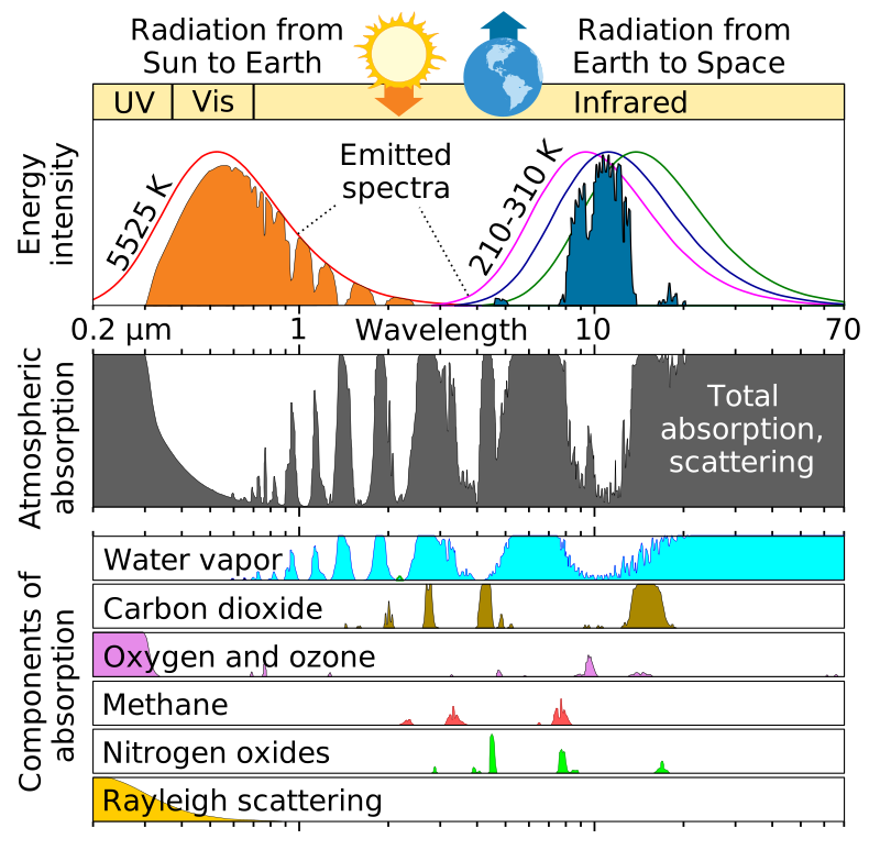
Introductory texts often summarize the atmosphere's transparency as three broad windows: the optical window (visible and near-infrared), the infrared windows (parts of the thermal infrared, chiefly 8 to 14 µm) and the radio window (microwave and radio, roughly 1 cm to 10 m or more). Everything between is blocked by gases, and the ionosphere reflects long radio waves.
Edges matter in multiple-choice items: the 8 µm end of the 8 to 14 µm window is still affected by water vapor, so the cleanest thermal window is about 10 to 12 µm. The 15 µm region is dominated by CO₂ but also lies on the wing of water vapor's rotation band, so keys sometimes list both gases as absorbers there. Earth emits mostly between about 4 and 40 µm with a peak near 10 µm; if a thermal-mapping question offers "1 to 10 µm" or "10 µm to 1 mm", choose the longer range.
Attenuation and the Beer-Lambert law
A beam passing through an absorbing or scattering medium loses the same fraction of its intensity in each equal step, so intensity decays exponentially. The attenuation (extinction) coefficient (also written or , in m⁻¹) says how quickly; the product is the optical depth (dimensionless), and is the transmittance. Final intensity is inversely, exponentially related to the coefficient. Along a slanted path the optical depth grows as , where is the angle from vertical; for an active sensor the beam goes down and back, so the two-way transmittance is .
Visibility follows the same physics: the Koschmieder relation gives visual range for a black target against the sky. In water, attenuation is strongly wavelength dependent: NIR is absorbed within centimeters, red within a few meters, and blue-green light (about 450 to 550 nm) penetrates deepest, tens of meters in clear ocean. That is why water looks blue, why underwater photos turn blue, why bathymetric lidar uses green light, and why ocean-color sensors work in blue and green bands.
In gas retrievals the law is often written with the absorber's amount: , with the mass absorption coefficient (m²/kg), the absorber density (kg/m³) and the path length (m). Inversion means solving for (the concentration) from the measured ratio : .
Refraction and the inverse-square law
Refraction is the bending of light as it crosses into a medium with a different speed of light. The refractive index measures how much the medium slows light: vacuum 1 exactly, air about 1.0003, ice 1.31, water 1.33, ordinary glass about 1.5, diamond 2.42. Refraction is described by Snell's law, , where the angles are measured from the surface normal. Light entering a denser medium (higher ) slows down and bends toward the normal; light entering a lower- medium speeds up and bends away. In remote sensing it matters for lenses, for light entering water (the bottom of a clear lake looks shallower than it is, a correction optical bathymetry must make) and for the slight bending of light through the atmosphere near the horizon. Division B treats Snell's law qualitatively: know which way the ray bends and why.
Related facts tests use:
- Total internal reflection: light going from high to low is trapped when the incidence angle exceeds the critical angle (48.6° for water to air, about 42° for glass to air). At incidence angles below the critical angle, it cannot occur. Total internal reflection inside snow and ice grains is one reason snow is so bright.
- Dispersion: is slightly larger for shorter wavelengths, so blue bends more than red. Refraction therefore decreases as wavelength increases, which splits white light in a prism (Newton's experiment) and makes rainbows.
- Atmospheric refraction and mirages: air's refractive index depends on density, so it falls with altitude and with higher temperature. Light bends through these gradients: a hot road under cooler air bends skylight upward into your eye, producing an inferior mirage that looks like water. The same gradients bend radar beams and lengthen GPS signal paths; GNSS radio occultation turns the measured bending into refractivity profiles, which give temperature and humidity.
- Seawater: its refractive index rises with salinity and falls as temperature rises, so warmer water bends a ray slightly less (a larger refraction angle).
The inverse-square law says irradiance from a point source falls as : double the distance and the power per unit area drops to a quarter, because the same power spreads over four times the area. It explains why the solar irradiance at Mars is less than half of Earth's and why an active sensor's echo is weak. Again, Division B asks about it qualitatively; Division C can use it in energy-balance arithmetic.
Refraction in optics and in the sky. A lens works by refraction: its refractive index and curvature set the focal length. Because the index changes with wavelength (dispersion), different colors focus at slightly different points (chromatic aberration), and each glass surface reflects a few percent of the light, so sensor optics use lens combinations and anti-reflection coatings. The green flash seen just as the Sun sets is also a refraction effect: the atmosphere refracts (bends) shorter wavelengths slightly more, so the green image of the Sun's rim sets last, while blue and violet are mostly scattered out of the long path.
Reflection and polarization
When light reaches a surface it is reflected, absorbed or transmitted, and the three fractions add to 1. How it reflects depends on roughness compared with the wavelength. Specular reflection from a smooth surface sends light off in one direction, with the angle of reflection equal to the angle of incidence (a mirror, calm water, a road for radar). Diffuse reflection from a rough surface spreads light in many directions; an ideal diffuse surface whose radiance is the same from every viewing direction is Lambertian, and for it radiance . Real surfaces are in between, described by the bidirectional reflectance distribution function (BRDF), which is why the same field looks brighter or darker depending on sun and view angles. A surface that is rough at visible wavelengths (sand) can be smooth for 20 cm radar waves; the usual rule (the Rayleigh roughness criterion) calls a surface smooth when its height variations are less than about , with the incidence angle.
Remote sensing names for special reflections:
- Sun glint (sunglint): specular reflection of sunlight off water straight into the sensor; it saturates pixels and hides what lies in and under the water, so ocean sensors tilt or mask it.
- Backscatter: energy scattered back toward the source, the quantity radar measures.
- Corner reflector: two or three perpendicular surfaces (building and street, ship hull and sea) bounce energy straight back toward the source, giving very bright radar returns (double bounce).
- Retroreflector: a prism array that returns light exactly along its incoming path; satellites such as Jason carry laser retroreflectors so ground lasers can measure their orbit.
- Albedo is the fraction of incoming solar radiation a surface reflects (0 to 1). Snow is bright because light meets thousands of air-ice interfaces between grains and is scattered back out before it can be absorbed; as grains grow with age or melt, there are fewer interfaces per centimeter and albedo drops, especially in the NIR. Clear, bubble-free ice has few interfaces and is much darker than white, bubbly ice or fresh snow.
Polarization describes the orientation of a light wave's electric field; only transverse waves can be polarized. Sunlight is unpolarized because it comes from countless independent emitters with random orientations. Light becomes polarized by reflection (fully so at Brewster's angle, about 53° from the normal for water, which is why polarized sunglasses cut horizontal glare), by scattering (Rayleigh-scattered skylight is most polarized about 90° from the Sun), by transmission through a polarizing filter or absorption (dichroic materials) and by refraction in birefringent crystals, which split a beam into two polarized rays. Polarization can be linear, circular or elliptical. Because aerosol and cloud particles of different size, shape and composition polarize light differently, polarimeters are used for aerosol studies: POLDER on PARASOL, and HARP2 and SPEXone on PACE. Lidar measures the depolarization of its echo: spherical droplets keep the laser's polarization, while irregular ice crystals, dust and ash depolarize it. Radar polarization channels (HH, HV, VH, VV) are covered under radar.
Radiometric quantities and units
Two radiometric words are often confused. Irradiance is power arriving per unit area of a surface, in W/m², with no direction attached. Radiance is power per unit area per unit solid angle, in W·m⁻²·sr⁻¹, so it describes what a sensor sees looking in one direction. A satellite measures radiance; a surface energy balance uses irradiance. Radiance does not change with distance along a ray in a clear medium (a wall looks equally bright from 1 m or 10 m, it just covers a smaller angle), while the irradiance from a small source falls as . A steradian (sr) is the unit of solid angle: , and a full sphere is sr.
| Quantity | Symbol | Unit | Meaning |
|---|---|---|---|
| Radiant energy | J | Total energy | |
| Radiant flux (power) | W | Energy per second | |
| Irradiance | W/m² | Flux arriving per unit area | |
| Radiant exitance | W/m² | Flux emitted per unit area ( for a blackbody) | |
| Radiosity | W/m² | Flux leaving per unit area, emitted plus reflected | |
| Radiant intensity | W/sr | Flux per solid angle from a point source | |
| Radiance | W·m⁻²·sr⁻¹ | Flux per area per solid angle in one direction | |
| Spectral radiance | W·m⁻²·sr⁻¹·µm⁻¹ | Radiance per unit wavelength; what each band measures | |
| Reflectance, albedo | none (0 to 1) | Reflected fraction of incident flux |
Radiometers are not limited to one band: they exist for ultraviolet, visible, near-infrared, thermal infrared (the most common for temperature) and microwave wavelengths. Atmospheric emission matters mainly in the thermal infrared and microwave, where gases and clouds radiate at their own temperature; in the visible and near-infrared the atmosphere affects the signal by scattering and absorption, not by emission.
Sensors and scanning
A sensor is active if it supplies its own energy and measures what comes back. Radar, lidar, laser altimeters and synthetic aperture radar are active. A sensor is passive if it only measures energy that already exists, either reflected sunlight or thermal emission from the surface and atmosphere. Optical cameras, multispectral imagers, infrared radiometers and most climate-monitoring radiometers are passive. The distinction is not about whether sunlight is involved: a camera photographing sunlit land is passive even though the light comes from the Sun. Mission details for every satellite named below are in the Satellites and instruments reference.
Every remote sensing system has the same chain of elements: (1) an energy source or illumination (the Sun, Earth's own thermal emission, or the sensor's own pulse); (2) radiation and the atmosphere, crossed on the way down and again on the way up; (3) interaction with the target (reflection, absorption, emission, scattering); (4) recording by the sensor; (5) transmission, reception and processing of the data, usually through a ground station; (6) interpretation and analysis; and (7) application to a real problem by the user. Questions that ask what limits a system usually point to one link in this chain.
Active and passive sensors classified
Tests love sorting lists. Use the energy source, not the wavelength or platform, to decide.
| Sensor or device | Class | Why |
|---|---|---|
| Camera without flash, human eye, binoculars | Passive | Records light already present |
| Camera with flash, phone Face ID or time-of-flight sensor | Active | Supplies its own light pulse |
| Thermal (infrared) camera, FLIR, infrared radiometer | Passive | Records emitted heat; works at night because the target emits |
| Night-vision goggles (image intensifier) | Passive | Amplifies faint existing light |
| Multispectral and hyperspectral imagers (OLI, MSI, MODIS, ASTER) | Passive | Reflected and emitted radiation |
| Radiometer, spectroradiometer, spectrometer (CERES, OCO-2) | Passive | Measures radiation intensity or spectrum |
| Sounders (CrIS, AIRS, Aura MLS) | Passive | Measure emitted IR or microwave in many channels to retrieve profiles (one archive key calls a sounder active; standard usage is passive) |
| Passive microwave radiometer (AMSR, GMI, SMAP radiometer) | Passive | Measures natural microwave emission as brightness temperature |
| Radio telescope, microphone | Passive | Receive only |
| Radar, SAR, InSAR (Sentinel-1, SRTM) | Active | Transmits microwave pulses |
| Radar altimeter (Jason), scatterometer (QuikSCAT) | Active | Transmits pulses, times or measures the echo |
| Precipitation and Doppler weather radar (GPM DPR, NEXRAD), cloud radar (CloudSat) | Active | Transmits pulses |
| Police speed gun | Active | Doppler radar or lidar |
| Lidar, laser altimeter (CALIOP, ICESat-2), laser fluorosensor | Active | Transmits laser pulses |
| Sonar | Active, but acoustic | Uses sound, not EM radiation, because water absorbs EM waves within meters |
| GPS receiver, GNSS radio occultation | Passive receiver | Uses signals transmitted by other satellites |
| Space gravimetry (GRACE) | Neither in the usual sense | Senses gravity; its microwave or laser link ranges between the two satellites, not to the ground |
| CALIPSO (as a satellite) | Both | Active lidar plus passive infrared and visible imagers |
A passive visible sensor cannot collect useful data at night because there is no sunlight to reflect, and it cannot see through cloud. A passive thermal sensor works day and night because the surface emits all the time, but clouds are opaque in the thermal infrared, so it measures cloud-top temperature instead of the surface under cloud. Passive microwave sensors see through most cloud but need huge antennas for fine detail, so their pixels are tens of kilometers. Active sensors control the wavelength, polarization and angle of their illumination, but they draw more power, cost more and often have shorter lives.
Detectors
A detector turns photons into an electrical signal that is digitized into digital numbers (DN). The choice of detector material sets which wavelengths a sensor can see.
| Detector | Wavelengths | Notes |
|---|---|---|
| Silicon CCD (charge-coupled device) | About 0.4 to 1.1 µm | Charge packets are shifted across the chip to one output; low noise; the classic satellite and camera detector |
| Silicon CMOS | About 0.4 to 1.1 µm | Each pixel has its own amplifier; faster, lower power |
| InGaAs photodiodes | About 0.9 to 1.7 µm (extended to about 2.5 µm) | SWIR |
| HgCdTe (mercury cadmium telluride) | SWIR to longwave IR, tunable | Must be cooled for thermal bands |
| InSb (indium antimonide) | About 1 to 5.5 µm | Midwave IR; cooled |
| Microbolometer, thermistor bolometer, thermopile | Broad thermal IR | Senses heating rather than counting photons; uncooled thermal cameras and broadband radiometers such as CERES |
Infrared detectors are cooled because a warm detector and its housing emit their own thermal radiation and dark current, which swamps a weak signal. A detector's quantum efficiency is the fraction of photons that produce an electron (external quantum efficiency counts all incident photons; internal counts only absorbed photons). The size and number of detector elements in an array set the spatial resolution and the number of pixels per line.
Thermal-infrared detectors such as mercury cadmium telluride must be cooled, typically to about 60 to 100 K, or their own heat swamps the signal. Early missions used stored cryogens (solid or liquid coolant) that boiled away, so the coolant supply set the mission's thermal lifetime; modern instruments use mechanical cryocoolers or passive radiators, but cryocooler wear or degradation can still end or limit a thermal channel (ASTER's SWIR bands failed in 2008 when their detector temperature could no longer be held).
An analog image is continuous, like a photograph on film, where tone varies smoothly and resolution is limited by film grain. A digital image is a grid of discrete pixels, each holding a number (DN) quantized to a fixed number of levels. Scanning a photo turns analog into digital; satellite sensors record digital images directly.
Radar imaging, interferometry and elevation models
RADAR stands for RAdio Detection And Ranging. Modern radars use microwaves (centimeter to millimeter wavelengths). They work day and night and see through cloud, smoke, and all but heavy rain, because the wavelength is far longer than cloud droplets. Radar bands carry letter names from World War II; learn the order and one example for each.
ReferenceMicrowave and radar bands· 9 rows
IEEE letter bands. Wavelength . Longer wavelengths penetrate vegetation, dry soil and rain better; shorter ones see smaller particles and finer surface roughness but are attenuated more by rain.
No rows match.
| Band | Frequency | Wavelength | Example instruments and uses |
|---|---|---|---|
| P | About 0.3 to 1 GHz | About 30 to 100 cm | Biomass radar (ESA BIOMASS); deepest canopy and soil penetration |
| L | 1 to 2 GHz | 15 to 30 cm | ALOS PALSAR, NISAR; SMAP radiometer at 1.4 GHz for soil moisture; GPS signals; sees through forest canopy and dry sand |
| S | 2 to 4 GHz | 7.5 to 15 cm | NEXRAD weather radar (about 10 cm, least rain attenuation); NISAR |
| C | 4 to 8 GHz | 3.75 to 7.5 cm | Sentinel-1 (5.405 GHz, 5.55 cm), RADARSAT, SRTM main radar (5.3 GHz), Jason second altimeter frequency, ASCAT scatterometer |
| X | 8 to 12 GHz | 2.5 to 3.75 cm | TerraSAR-X, SRTM second radar (X-SAR), short-range weather radars; attenuated by heavy rain |
| Ku | 12 to 18 GHz | 1.67 to 2.5 cm | Jason and TOPEX main altimeter (13.6 GHz), GPM DPR KuPR (13.6 GHz), QuikSCAT SeaWinds |
| K | 18 to 27 GHz | 1.1 to 1.67 cm | Includes the 22.2 GHz water-vapor line; GRACE inter-satellite ranging (K and Ka) |
| Ka | 27 to 40 GHz | 0.75 to 1.1 cm | GPM DPR KaPR (35.5 GHz), SWOT KaRIn; light rain and snow |
| W | 75 to 110 GHz | 2.7 to 4 mm | CloudSat Cloud Profiling Radar (94 GHz); cloud droplets |
The name letters do not follow wavelength order, so memorize "P L S C X Ku K Ka (V) W" from longest to shortest.
Side-looking geometry is a strength, not only a necessity: the oblique illumination creates shading and radar shadow that exaggerate relief, so side-looking radar images bring out faults, folds, drainage and other terrain structure for geologists, and their texture helps map forest and land use.
Radar geometry, resolution and distortions
An imaging radar looks sideways (side-looking airborne radar, SLAR), because a nadir-looking radar could not tell apart two points at equal distances on either side of the track. Terms: range is the across-track direction (perpendicular to flight); azimuth is the along-track direction (parallel to flight); slant range is the line-of-sight distance; ground range is the horizontal distance; near range is the side closest to the track and far range the farthest. The look angle is measured at the radar from vertical; the incidence angle is measured at the ground between the beam and the local vertical (or normal), and the depression angle is measured from horizontal (depression = 90° − look angle on a flat Earth).
Range resolution depends on pulse length: two targets are separated only if their echoes do not overlap, so they must be at least half a pulse length apart in slant range. Short pulses give fine resolution but carry little energy; real radars send a long pulse whose frequency sweeps across a bandwidth (a chirp) and then compress it in processing (pulse compression), giving resolution . Azimuth resolution of a real-aperture radar is the beam's footprint width, , which grows with distance and shrinks with a longer antenna. A synthetic aperture radar (SAR) uses the platform's motion to combine many echoes from one spot coherently, imitating an antenna hundreds of meters to kilometers long, so it reaches meter-to-tens-of-meters detail from orbit, day or night and through cloud. Remarkably, a SAR's azimuth resolution is about half its real antenna length, independent of range and wavelength. Seasat (1978) was the first civilian Earth-observing satellite to carry an imaging SAR.
Side-looking geometry distorts mountains, and the three distortions are frequently tested:
- Foreshortening: a slope facing the radar appears compressed and bright, because its top is only a little farther from the radar than its base. Worst in mountains and at small incidence angles.
- Layover: an extreme case. When the slope facing the radar is steeper than the incidence angle, the radar pulse reaches the peak before the base, so the top is imaged closer to the radar than the bottom and the mountain appears to lean toward the sensor.
- Radar shadow: a slope facing away that is steeper than the depression angle receives no energy and appears black. Shadow grows at large incidence angles (far range); layover is worse at small incidence angles (near range).
- Slant-range scale distortion: in an image displayed in slant range, near-range features are compressed relative to far-range ones; converting to ground range corrects it.
Speckle is the grainy "salt and pepper" texture of every radar image. It comes from coherent interference of echoes from many small scatterers within one pixel, not from the ground itself. It is reduced by multi-look processing (averaging several independent looks) and by spatial filtering, both at the cost of resolution.
Slant range versus ground range. A side-looking radar measures slant range , the straight-line distance from the antenna to the target. On flat ground the horizontal ground range is (equivalently , with the radar's height and the look angle from vertical). In a slant-range image, features in the near range are compressed relative to the far range (slant-range scale distortion); resampling each pixel to ground range removes the compression. Example: km and km give km.
Clutter and jamming. Clutter is unwanted echo of the radar's own pulse from things you are not trying to measure (ground, sea waves, buildings, insects in a weather radar). Jamming is interference from an outside transmitter on the radar's frequency, deliberate or accidental, that masks the real echoes.
Backscatter: roughness, moisture and polarization
An imaging radar records backscatter, the fraction of its pulse returned toward the antenna, usually expressed as the backscatter coefficient in decibels. Smooth surfaces such as calm water and runways act like mirrors and send the pulse away, so they look dark. Rough surfaces (forest canopy, plowed fields, rough seas) scatter some energy back and look medium-bright. Buildings and steep slopes facing the radar form corner reflectors and look very bright. Wet soil returns more than dry soil because water raises the surface's dielectric constant: dry soil has a dielectric constant of about 3 to 5, wet soil 20 or more and liquid water about 80. The same physics lets passive microwave radiometers map soil moisture (wet soil has lower microwave emissivity and looks colder) and tell sea ice from open water.
Each surface sends radar energy back by a dominant mechanism, and each mechanism is brightest in particular polarization channels:
| Scattering mechanism | Where it happens | Strongest in |
|---|---|---|
| Specular (mirror) | Calm water, smooth pavement, flood water | Very dark everywhere |
| Surface (single bounce, diffuse) | Bare soil, rough sea, sand | Like-polarized VV (or HH) |
| Double bounce | Buildings and streets, tree trunks standing in flood water, ships | Very bright HH |
| Volume | Forest and crop canopies, dry snow | Cross-polarized HV or VH |
| Helix | Complex urban structures (in polarimetric decompositions) | Fully polarimetric data |
A radar transmits and receives in horizontal (H) or vertical (V) polarization. Like-polarized (co-pol) channels are HH and VV; cross-polarized channels are HV and VH. A single-pol system records one channel (HH or VV), dual-pol records one transmit with both receives (for example VV + VH, Sentinel-1's standard mode over land), and quad-pol (fully polarimetric) records all four. VV is most sensitive to surface roughness, so it maps ocean wind and soil roughness; HH penetrates canopies better and highlights double bounce (flooded forest, mangroves); VH and HV come mostly from multiple scattering in vegetation, which depolarizes the wave, so cross-pol is bright over forest and nearly black over smooth water. Longer wavelengths penetrate farther: L-band passes through forest canopy to the trunks and ground and through meters of hyper-dry sand (Shuttle radar revealed buried river channels in the Sahara), while X-band returns mostly from the top of the canopy. Clear-cuts look darker than the forest around them because they lose the canopy's volume scattering; texture is the main clue for forest type in radar images.
Interferometry and elevation models
Interferometric SAR (InSAR) compares the phase of two SAR images. Phase differences come from topography (if the two views are from slightly different positions, as in SRTM) or from ground motion between two dates. An InSAR change map shows colored fringes; each full color cycle is a fixed amount of motion toward or away from the satellite (half the radar wavelength, about 2.8 cm for Sentinel-1). Tightly packed fringes mean a lot of motion, for example a swelling volcano, a fault after an earthquake or a city sinking as groundwater is pumped. Division B tests InSAR at this interpretive level only. Radargrammetry instead uses two images of the same area from different incidence angles, like a stereo photo pair.
A digital elevation model (DEM) is a grid of ground heights. SRTM flew a radar interferometer on the Space Shuttle in February 2000 and produced a near-global DEM; ASTER stereo images produced another. Subtracting an older DEM from a newer one shows where material was removed (a landslide scar, a quarry, a retreating glacier) and where it piled up. A DEM that includes treetops and buildings is a digital surface model (DSM); one with them removed is a digital terrain model (DTM). Lidar is especially good at both because it records multiple returns.
Radar altimetry and scatterometry
A radar altimeter points straight down (nadir) and times the echo. The surface height above a reference ellipsoid is the satellite's orbital height (known to centimeters from DORIS, GPS and laser tracking) minus the measured range and minus corrections. Over the ocean the mean surface follows the geoid, the equipotential surface of gravity that approximates mean sea level, plus currents and tides; altimetry measures sea surface height, wave height and wind, and over land and ice it measures ice-sheet and lake levels and subsidence. It cannot measure sea surface temperature.
Wind speed comes from the strength of the nadir echo: wind roughens the sea with short waves, which scatter the pulse away from the vertical, so the backscatter coefficient σ⁰ falls as wind speed rises. Early altimeters (Skylab, GEOS-3 and Seasat, 1973 to 1978) first showed this, and wind is retrieved with empirical relations of the form (σ⁰ in linear units, the wind speed, and fitted constants; side-looking scatterometers use a similar power law that increases with wind).
Every correction tests ask about:
- Ionospheric delay: free electrons slow the signal by an amount proportional to , so the range looks too long. Measuring at two frequencies (Ku 13.6 GHz and C 5.3 GHz on TOPEX and Jason) lets the delay be computed and removed.
- Wet troposphere: water vapor also slows the signal. A passive microwave radiometer on board (Jason's AMR near 18.7, 23.8 and 34 GHz; TOPEX used 18, 21 and 37 GHz, with 21 GHz as the water-vapor channel) measures it.
- Dry troposphere (from surface pressure models), sea-state bias, tides and the inverse barometer effect are removed with models.
The returned waveform carries three signals: the timing of its leading edge gives the range to mean sea level, the slope of the leading edge gives significant wave height (rough seas smear the echo), and the strength of the return gives wind speed (a smooth sea is brighter at nadir). Altimeters have a small field of view and see only the area directly beneath them; over land, steep slopes and rough terrain degrade accuracy. Jason-class altimeters measure global sea level to a few centimeters per measurement; averaging many measurements gives rise rates of millimeters per year. Laser altimeters (ICESat-2) do the same with light, which suits ice and vegetation but not cloudy skies.
A scatterometer is a radar that measures backscatter (not range) from the sea surface at several angles. Because wind-driven ripples set the backscatter, it retrieves ocean surface wind speed and direction (QuikSCAT's SeaWinds, ASCAT). Long-pulse scatterometers view large areas at once, trading resolution for coverage.
The altimeter's footprint is the patch of surface its pulse illuminates. For pulse-limited ocean altimeters such as Jason it is a few kilometers across (about 2 to 10 km, larger in high seas), much smaller than the beam-limited footprint the antenna alone would give; SAR-mode altimeters (CryoSat-2, Sentinel-6) sharpen it to about 300 m along track.
Altimeters save transmitter power with pulse compression: instead of a very short, high-power pulse they send a longer, lower-power frequency-swept pulse (a chirp) and compress the echo in processing, which gives the range resolution of a short pulse; on-board waveform tracking and averaging of many echoes further reduce the power needed. QuikSCAT (1999 to 2009), a Ku-band scatterometer that mapped ocean wind speed and direction, flew in a polar sun-synchronous orbit (about 800 km) with an 1,800 km swath, because global daily coverage of the oceans needs a near-polar orbit.
Weather, precipitation and Doppler radar
A precipitation radar sends pulses into clouds and measures the echo power from raindrops, snow and hail at each range, giving a 3D picture of precipitation. Echo strength is expressed as the reflectivity factor , which for small drops grows as the sixth power of drop diameter, so a few large drops dominate. It is reported in dBZ (): roughly 20 dBZ is light rain, about 40 dBZ heavy rain, and above 50 to 55 dBZ suggests hail. Rain rate is estimated from a Z-R relationship (a common one is , with in mm/h). Liquid water returns about five times as much power as ice of the same size, so melting snow produces a bright band; hail's large echoes can make rain look heavier than it is. Radar cannot measure rain temperature.
NEXRAD is the U.S. network of about 160 WSR-88D ground Doppler radars (S band, about 10 cm wavelength, so heavy rain barely attenuates the beam). It scans a series of elevation angles every few minutes. Base reflectivity is the reflectivity from a single tilt, usually the lowest (0.5°), shown out to about 230 km (124 nautical miles), with a long-range version out to about 460 km (248 nautical miles). Composite reflectivity is the maximum reflectivity found at any elevation angle above each point, out to about 230 km; it shows the strongest cores in a storm, including hail aloft that base reflectivity can miss. Base velocity gives the radial (toward or away) speed of targets, out to about 230 km. Because the beam rises with distance and Earth curves away, distant radar echoes come from high in the storm and low clouds far away are missed.
Wavelength choice is a trade-off. Short wavelengths (Ka, W) detect small cloud and drizzle particles (CloudSat's 94 GHz radar, nadir-pointing) but are strongly attenuated by heavy rain; long wavelengths (S band, as in the US NEXRAD network) pass through heavy rain with little attenuation. Attenuation (loss of signal through the rain itself) is worst for X, Ku and Ka bands. GPM's Dual-frequency Precipitation Radar (Ku 13.6 GHz and Ka 35.5 GHz) compares the two frequencies, which respond differently to large and small drops, to estimate drop size distribution and to separate rain from snow.
Doppler radar also measures the frequency shift of the echo, which gives the speed of raindrops toward or away from the radar (the radial velocity); side-by-side inbound and outbound velocities (a velocity couplet) reveal rotation in a storm, while the hook echo is a reflectivity signature. A shift to higher frequency means motion toward the radar; lower frequency means motion away. One Doppler radar measures only the radial component, so two or more radars are needed to map the full horizontal wind. Dual-polarization radar transmits and receives both horizontal and vertical pulses, so it can tell drop shape and precipitation type (rain, hail, snow, even insects and smoke). Airborne Doppler radars on hurricane hunter aircraft map storm winds, and satellite radars are not blocked by terrain.
Received power falls very steeply with distance because the pulse spreads out on the way to the target and the echo spreads out again on the way back: the radar equation gives , where is antenna gain and the target's radar cross section. Doubling the range cuts the echo to 1/16. The wave's speed does not appear.
Lidar
Lidar (LIght Detection And Ranging) times laser pulses instead of radio pulses, so it maps heights and cloud or aerosol layers with fine vertical detail but cannot see through thick cloud. It is the laser counterpart of radar. A system has a laser, a scanner, a receiver telescope and detector, and, on aircraft, a GPS receiver and an inertial measurement unit (IMU, which measures roll, pitch and yaw) to locate every return. Most lidars fire many thousands of pulses per second (150 kHz = 150,000 pulses per second), building a point cloud of x, y, z coordinates, each with an intensity (return strength, which depends on surface reflectance but also on range, angle and roughness, so it is hard to calibrate).
| Lidar type or wavelength | Use |
|---|---|
| 1,064 nm (NIR) | Topographic mapping and vegetation; leaves and land reflect NIR strongly; GEDI on the ISS |
| 532 nm (green) | Bathymetry (green penetrates clear water); ICESat-2's photon-counting altimeter; CALIOP's polarization channel |
| 532 + 1,064 nm | CALIOP on CALIPSO: the color ratio separates large particles (similar returns) from small aerosol (much weaker at 1,064 nm) |
| 355 nm (UV) | Doppler wind lidar (ESA Aeolus, 2018 to 2023), measuring wind from the Doppler shift of molecular and aerosol backscatter |
| DIAL (differential absorption lidar) | Two wavelengths, one on and one off a gas absorption line; the difference gives gas concentration profiles (ozone, water vapor, CO₂) |
| Raman lidar | One laser; detects inelastic Raman-shifted light from specific molecules (water vapor, N₂) |
| HSRL (high spectral resolution lidar) | Separates molecular from aerosol backscatter to measure aerosol extinction directly |
A single pulse over forest returns several echoes: the first return from the canopy top, intermediate returns from branches and the last return from the ground, so tree height is the first-return elevation minus the last-return elevation. Bathymetric lidar compares the green echo from the water surface with the echo from the bottom; it works best in shallow, clear water and fails in deep or turbid water. Depolarization of the echo tells particle shape: spherical liquid droplets do not depolarize, irregular ice crystals, dust and volcanic ash do. Lidar often flies at night because sunlight adds background noise to the faint returns. Lidar's short wavelength gives much finer resolution and less noise than radar and maps canopy height and terrain under trees, but clouds, fog and heavy rain block it and it needs a clear line of sight; radar is better through weather and for large areas and storms. Photogrammetry (stereo photos) is cheaper but cannot see the ground under a canopy.
More lidar details tests ask. Differential absorption lidar (DIAL) fires two wavelengths, one on a gas's absorption line and one just off it, and uses the ratio of their returns to get that gas's concentration along the path; because both pulses share the same optics and atmosphere, most instrument and aerosol effects cancel. Raman lidar detects light scattered at a shifted wavelength by a specific molecule (water vapor, nitrogen); the Raman return is about a thousand times weaker than the elastic return, so it needs narrowband filters or a spectrometer to block the elastic line and works best at night. Lidar lasers include solid-state Nd:YAG (1,064 nm and doubled 532 nm) and gas excimer lasers for the ultraviolet (XeCl at 308 nm, XeF at 351 nm). For airborne mapping, the number of points on a target is its area times the point density (times the returns per pulse if density is quoted per pulse): a tree crown 3 m in radius at 30 points per m² gets points. Beyond elevation and canopy height, lidar is used for obstacle detection and collision avoidance on self-driving cars and drones, and for wind (Doppler lidar).
Micropulse lidar (MPL, used in NASA's MPLNET ground network) fires very low-energy pulses (microjoules) thousands of times per second, so it is eye-safe and can run unattended around the clock to profile clouds and aerosols.
Space gravimetry
Space-based gravimetry (Division C, GRACE and GRACE-FO) does not sense light at all. Two identical satellites fly in the same low polar orbit about 220 km apart and measure changes in their separation to within about 10 micrometers (micron level) with a K- and Ka-band microwave ranging link (GRACE-FO adds a laser ranging interferometer); accelerometers remove non-gravitational forces such as drag. As the pair approaches a region of extra mass (an ice sheet, a full aquifer), the leading satellite is pulled forward first and speeds up, so the gap widens; then the trailing one is pulled and catches up; past the mass, the leader is slowed. Over a region that has lost mass (a depleted aquifer), the pull is weaker and the leader accelerates less. Monthly maps of these changes show mass moving: ice-sheet loss, groundwater depletion (California's Central Valley, northern India), ocean mass gain and seasonal water storage. GRACE measures mass, so it misses thermal expansion of seawater; how this feeds sea-level budgets is covered in the climate chapter. The underlying principle is Newton's law of gravitation, .
Gravity is measured as an acceleration, in m/s² (standard surface value about 9.81 m/s²). Geophysicists also use the Gal (after Galileo): 1 Gal = 1 cm/s² = 0.01 m/s², so 1 milligal (mGal) = 10⁻⁵ m/s², about one-millionth of Earth's surface gravity. GRACE's month-to-month gravity changes are tiny (on the order of microgals, µGal), so monthly maps are usually converted to equivalent water thickness in centimeters.
Three tracking modes exist. High-low satellite-to-satellite tracking: high GPS satellites track a single low satellite (CHAMP, 2000). Low-low tracking: two satellites in the same low orbit range to each other (GRACE, GRACE-FO). Gravity gradiometry: accelerometers inside one satellite measure the difference in gravity across the spacecraft (ESA's GOCE, 2009 to 2013), which gives the finest static gravity field.
Scanning systems
A satellite builds an image by moving and sampling. A whiskbroom (across-track) scanner uses a rotating or oscillating mirror to sweep detectors across the track, one ground spot at a time, while the platform moves forward. A pushbroom (along-track) scanner uses a line of detectors, one per cross-track pixel, that images an entire strip at once; the platform's motion builds the second dimension. Pushbroom designs have no moving mirror, so each pixel is viewed longer, but they need many detectors calibrated against each other. A framing camera captures a whole two-dimensional scene at once, as eyes and ordinary cameras do.


| Feature | Whiskbroom (across-track) | Pushbroom (along-track) |
|---|---|---|
| How a line is built | Rotating or oscillating mirror sweeps a few detectors side to side, perpendicular to the flight direction | A linear array (one detector per pixel across the swath, perpendicular to flight) records the whole line at once |
| Moving parts | Yes (mirror) | None |
| Dwell time per pixel | Short (the line time is shared among all pixels in the line) | Long (each detector stares for the whole line time), so better SNR |
| Calibration | Few detectors, easy to keep uniform | Thousands of detectors; mismatches cause along-track striping |
| Swath | Can be very wide (MODIS about 2,330 km) | Limited by optics and array length |
| Geometric distortion | Panoramic distortion toward swath edges | Less; distortion only across the line |
| Examples | Landsat MSS, TM, ETM+; MODIS; AVHRR | Landsat 8 and 9 OLI and TIRS, Sentinel-2 MSI, ASTER VNIR, SPOT |
Through Landsat 7, every Landsat scanning imager (MSS, TM, ETM+) was a whiskbroom (Landsats 1 to 3 also carried RBV framing cameras); Landsat 8 introduced pushbroom sensors. Modern missions prefer pushbroom designs because there is no mirror to wear out, they are smaller and lighter, and the longer dwell time raises the signal-to-noise ratio. Dwell time is calculated in the coverage section below.
Geometric distortions of scanned and photographed images
- Panoramic (tangential scale) distortion: a whiskbroom mirror sweeps at a constant angle per step, but the ground distance per step grows toward the swath edges, because the sensor is farther away and looks obliquely. Pixels near the edge cover more ground, so features there are compressed in the image and straight lines can bend into S shapes. Off-nadir resolution is therefore degraded.
- Relief displacement: tall objects lean away from nadir. In a vertical aerial photograph they lean radially away from the photo center (at the exact center you see only rooftops); in a scanner image they lean away from the nadir line, perpendicular to the track. An orthophoto has relief displacement removed, so it has uniform scale.
- Skew distortion: Earth rotates eastward under the satellite while a scene is built line by line, so each line is offset slightly west of the previous one and the image is skewed; it is corrected by deskewing.
- Platform motion: roll, pitch, yaw and altitude changes shift lines; aircraft carry IMUs to correct them.
- Scan-line gaps and striping: Landsat 7's scan line corrector failed on May 31, 2003, leaving wedge-shaped gaps (about 22% of each scene) that widen toward the scene edges. Uneven detectors cause striping (every 16th line in TM, along-track stripes in pushbroom images), removed by destriping.
- Radar distortions (foreshortening, layover, shadow, slant-range compression) are listed in the radar section above.
Imagers, radiometers and spectrometers
An imager forms an image in several bands. A multispectral imager records a handful of broad bands. A radiometer measures radiance or irradiance in a few broad channels without necessarily forming a detailed image, as climate instruments do. A spectrometer records many narrow bands and identifies composition from the shape of the spectrum. A spectroradiometer (such as MODIS, the Moderate Resolution Imaging Spectroradiometer) combines both: calibrated radiance in many bands. An optical imager records reflected visible and near-infrared light, so it needs daylight and gives fine detail; an infrared (thermal) imager records emitted heat, so it works at night and shows temperature but has coarser pixels (longer wavelengths, fewer photons). A sounder measures radiance in many channels spread across an absorption band; each channel "sees" a different altitude, so together they retrieve vertical profiles of temperature, humidity or gases (CrIS on Suomi NPP, AIRS on Aqua).
Microwave instruments come in the same classes. Passive microwave radiometers (imagers) measure the brightness temperature of naturally emitted microwaves: AMSR-E and AMSR2, GMI on GPM and the SMAP radiometer map rain, sea ice, soil moisture and sea-surface temperature through cloud. Passive microwave sounders use many channels on the edges of the oxygen (near 50 to 60 GHz and 118 GHz) and water-vapor (22 and 183 GHz) absorption lines to retrieve temperature and humidity profiles (AMSU and ATMS looking down; MLS on Aura looking at the limb). The altimeter's on-board water-vapor radiometer (Jason's AMR) is another passive microwave radiometer. Microwave spectrometers in the strict sense are rare on these lists; limb sounders such as MLS resolve individual emission lines. Active microwave instruments are radars, scatterometers and altimeters.
A Crookes radiometer (the 'light mill' sold as a toy) is a partial-vacuum bulb with vanes black on one side and silver on the other. Light or infrared heats the black faces more, and gas molecules rebounding from the warmer faces (mostly near the vane edges, an effect called thermal transpiration) push them, so the vanes spin with the black sides trailing (moving away from the light). It spins faster in brighter light, but it is a demonstration of thermal gas effects, not a measuring instrument and not radiation pressure (radiation pressure alone would push the shiny sides harder).
Rule of thumb for classification questions: a sensor that outputs a number (radiance or a temperature reading) rather than a picture is a radiometer, such as a handheld infrared thermometer or CERES; one that builds a picture is an imager (or imaging radiometer); one that splits the light into many narrow bands is a spectrometer. Measuring snow depth or snow water equivalent needs an active technique (lidar or radar altimetry from two dates, snow-free minus snow-covered) or passive microwave scattering; measuring snow albedo is passive, so a mission doing both needs both kinds of sensor.
Spectral classes of imagers
Imagers are classed by how many bands they record and how narrow those bands are; more bands identify materials better but leave less light per band.
| Class | Bands | Bandwidth | Example | Trade-off |
|---|---|---|---|---|
| Panchromatic | 1 broad band (often 0.5 to 0.9 µm) | Very wide | Landsat 8 band 8 (15 m), black-and-white aerial film | Measures brightness only, but collects the most light per pixel, so it has the finest spatial resolution and smallest data volume |
| Multispectral | About 3 to 10 (some up to about 15) | Broad, separated | Landsat TM and OLI, Sentinel-2 MSI | General land cover and vegetation |
| Superspectral | More than about 10, often dozens | Narrower | MODIS (36 bands; also called multispectral) | Many targeted bands |
| Hyperspectral | Hundreds | Narrow (about 10 nm), contiguous | AVIRIS (224 bands), Hyperion, PACE OCI, EMIT | Full spectrum per pixel; identifies minerals, gases and plant species; huge data, lower SNR per band |
| Ultraspectral | Thousands | Very narrow | Infrared sounders such as AIRS (2,378 channels) and CrIS | Gas retrievals and profiles |
Higher spectral resolution means more, narrower bands; it identifies materials by narrow absorption features (minerals, gases), but each band collects less light, lowering SNR and often forcing larger pixels. Normal color film and sensors have blue, green and red layers, so there is no separate yellow layer; color in images of invisible wavelengths is assigned in processing (false color). Elements of image interpretation, band combinations and spectral indices are covered in the Division B map and image chapter.
Label questions: a sensor with a handful of broad bands (Landsat OLI, Sentinel-2 MSI) is multispectral; tens of bands (MODIS's 36) are sometimes called superspectral; hundreds of narrow contiguous bands (PACE OCI, Hyperion) are hyperspectral. If both "multispectral" and "superspectral" are offered for MODIS, "superspectral" is the more specific answer; if only multispectral and hyperspectral are offered, MODIS is multispectral.
Spectroscopy and gas retrieval
Spectra come in three basic types, described by Kirchhoff's rules of spectroscopy: a continuous spectrum from a hot dense source (a blackbody curve, the Sun's photosphere, a lamp filament), an emission spectrum where a hot, low-density gas emits only at particular wavelengths (bright lines on a dark background, like a neon sign), and an absorption spectrum where a cooler gas removes particular wavelengths from a continuous background (dark lines, like the solar spectrum's Fraunhofer lines or sunlight that has crossed Earth's atmosphere). Gas identification relies on absorption features. Each line exists because an electron, vibration or rotation jumps between quantized energy levels, and the photon's frequency equals the energy difference divided by . For hydrogen's visible Balmer series, with m⁻¹: the drop from to gives 410 nm (violet). Heavier hydrogen-like ions (He⁺, Li²⁺) have energy levels scaled by , so the same jump emits shorter wavelengths.
A band ratio divides one band by another (NDVI is a normalized version). Ratios cancel brightness differences caused by slope and shadow, and they isolate features: a ratio of a band inside a gas's absorption line to a nearby band outside it measures how much of that gas lies along the path. OCO-2 uses this idea in the 1.6 and 2.06 µm CO₂ bands, with an oxygen band as reference for the air column. A deeper absorption dip means more gas along the path, but clouds, aerosols, surface reflectance and viewing geometry also change the path length, so retrievals must account for them. The Division C list names atmospheric interactions with the terrestrial biosphere: plants draw down CO₂ each Northern Hemisphere summer and release it in winter (seen in OCO-2 maps), wetlands emit methane (seen by TROPOMI), fires release CO and aerosol, and healthy leaves emit a faint solar-induced fluorescence in the far red, which OCO-2's spectrometer retrieves near 760 nm as a measure of photosynthesis.
Viewing geometry: nadir, limb, occultation and multi-angle
Where a sensor points decides what it can measure: straight down for the surface and total columns, through the limb for thin layers and vertical profiles.
| Geometry | How it looks | Good for |
|---|---|---|
| Nadir | Straight down | Surface imaging, total columns, altimetry |
| Off-nadir pointing | Tilted toward a target | Faster revisit of one place (ASTER, commercial imagers) |
| Limb | Through the atmosphere's edge toward the horizon | Long path through thin layers, so high sensitivity to trace gases and sharp vertical profiles (Aura MLS); poor horizontal detail |
| Occultation | Looks at the Sun, a star or a GPS satellite through the limb as it sets or rises | Very accurate profiles from the attenuation or bending of the signal |
| Multi-angle | Views each spot from several angles (MISR on Terra: 9 cameras) | Aerosol type, cloud height, surface structure (BRDF) |
| Conical scan | Constant incidence angle around a cone | Passive microwave imagers (GMI on GPM) |
Image processing pipeline
Raw data pass through standard steps before analysis. Tests ask what each step does.
- Radiometric correction and calibration: convert DN to radiance using the sensor's gain and offset, then to top-of-atmosphere reflectance using sun angle and Earth-Sun distance; remove striping and detector differences. Sensors are calibrated before launch, by onboard sources (lamps, solar diffusers, blackbodies) and by vicarious calibration over stable, bright, uniform desert sites (Libya-4, Railroad Valley Playa), which also tracks slow drift over years.
- Atmospheric correction: remove scattering and absorption to get surface reflectance, using models (radiative transfer codes such as MODTRAN) or simple image-based methods such as dark object subtraction.
- Geometric correction: remove distortions and register the image to map coordinates with ground control points; orthorectification also uses a DEM to remove relief displacement.
- Enhancement: a histogram shows how many pixels have each DN; a contrast stretch spreads the used DN range over the full display range; density slicing groups ranges of DN into one color; low-pass filters smooth noise and speckle, high-pass filters sharpen edges; pansharpening merges a sharp panchromatic band with coarser color bands.
- Transformation: band ratios and indices, principal component analysis (compresses correlated bands into a few new ones), and composites.
- Classification and change detection: covered in the Division B chapter.
Ground-based measurements taken at the same time as the overpass (ground truth) are used to calibrate and validate satellite products.
Film versus digital, and long records. Photographic film records only about 0.3 to 0.9 µm in at most three broad emulsion layers, cannot sense SWIR or thermal infrared and is hard to calibrate; digital detectors cover the SWIR and thermal ranges in many narrow, calibrated bands. A climate data record spanning decades has to be stitched from several satellites, so the missions must overlap and be cross-calibrated against each other (and against stable references such as desert calibration sites) so that a change of instrument is not mistaken for a climate trend.
A mosaic is a single seamless image stitched from several overlapping scenes or flight lines, after each is georeferenced and its brightness balanced so the seams do not show; national and global base maps (and Google Earth) are mosaics of many dates.
Orbits and satellites
Satellites stay in orbit because gravity supplies the centripetal force that bends their path around Earth. The orbit's altitude sets its period, how much of the planet it sees at once and how fine its detail can be. Both divisions list orbit types by name, but the lists differ: Division B names low, medium and high Earth orbit, polar and non-polar, geostationary and geosynchronous; Division C adds sun-synchronous and uses the abbreviation HEO. Which orbit each named mission flies is in the Satellites and instruments reference; this chapter is the physics and the orbit types.
| Orbit | Typical altitude | What it is good for | Examples |
|---|---|---|---|
| Low Earth orbit (LEO) | About 160 to 2,000 km; most imagers fly near 700 to 830 km | Fine spatial detail, frequent passes, low launch cost; but drag shortens life and each satellite sees a small area | Landsat, Sentinel-2, Terra, Aqua, Suomi NPP, the ISS |
| Medium Earth orbit (MEO) | About 2,000 to 35,786 km | Wide coverage with a modest number of satellites | GPS (about 20,200 km), Galileo |
| Geostationary (GEO) | 35,786 km, over the equator | Hovers over one spot, so continuous imaging of one hemisphere | GOES |
| Geosynchronous | Period of one sidereal day (GEO is the equatorial, circular case) | Returns to the same sky position each day; an inclined one traces a figure eight | Communications satellites |
| High Earth orbit | Above geostationary altitude (beyond 35,786 km) | Very wide views, few satellites; some science and relay missions | Space-weather monitors |
| Highly elliptical | Low perigee, apogee tens of thousands of km | Slow near apogee, so long dwell over high latitudes | Molniya-type communications orbits |
| Polar | Usually LEO, inclination near 90° | Passes over both poles, so every latitude is eventually covered | Many Earth observers, GRACE |
| Sun-synchronous | LEO, inclination about 98° | Crosses each latitude at the same local solar time, so lighting is consistent | Terra (about 10:30 a.m.), Aqua and Suomi NPP (about 1:30 p.m.) |
| Non-polar (inclined) | LEO at moderate inclination | Concentrates passes on the tropics and mid-latitudes; varying overpass times | ISS (51.6°: ECOSTRESS), GPM core (65°), Jason (66°) |
Kepler's laws and orbital calculations
Kepler's laws describe every such orbit. (1) Orbits are ellipses with the central body at one focus (a circle is the special case of zero eccentricity; parabolas and hyperbolas are unbound paths). (2) A line from the central body to the satellite sweeps equal areas in equal times, so the satellite moves fastest at perigee and slowest at apogee. (3) The square of the period is proportional to the cube of the semi-major axis. The third law depends only on the central body's mass, not the satellite's, so every satellite at the same altitude has the same period.
Eccentricity runs from 0 (circle) toward 1 (very elongated). Earth's orbit around the Sun has , Venus about 0.007 (the most circular planetary orbit), Mars about 0.093 and Mercury about 0.21; Neptune's large moon Triton has an almost perfectly circular (but retrograde) orbit. A Molniya orbit has . For an ellipse, perigee distance , apogee distance , and the semi-minor axis .
Ellipse vocabulary: the semi-major axis is half the longest diameter; the semi-minor axis is half the shortest; the foci are the two points inside the ellipse (Earth sits at one); eccentricity measures elongation, from 0 (circle) toward 1. The closest point to Earth is perigee and the farthest apogee (around the Sun, perihelion and aphelion; in general, periapsis and apoapsis). Inclination is the angle between the orbit plane and the equator: 0° is equatorial, 90° polar, below 90° prograde (moving eastward with Earth's rotation) and above 90° retrograde.
Division C may calculate with Kepler's third law; Division B treats it qualitatively (higher orbit, longer period). The law also gives a ratio method that skips the constants. If one orbit's radius is 4 times another's, its period is times longer. A planet at 4 AU has an 8-year period if one at 1 AU has 1 year.

Sun-synchronous orbits and equator crossing times
A sun-synchronous orbit is slightly retrograde, which makes Earth's equatorial bulge swing the orbit plane eastward by about 1° per day (360° in a year, 0.986° per day), matching the Sun's apparent motion. Consistent local time matters because comparing two dates only means something if shadows and sun angle are similar. Sun-synchronous satellites fly at about 600 to 800 km with inclinations near 98°, so they are near-polar but never pass exactly over the poles. They are not always in sunlight (except special dawn-dusk orbits such as Sentinel-1's, which ride the day-night line).
A sun-synchronous orbit is described by its equator crossing time. A descending node is a north-to-south crossing; an ascending node is south-to-north. Morning satellites (Terra about 10:30, Landsat about 10:00, Sentinel-2 about 10:30) cross southbound on the day side, before afternoon clouds build over land. Afternoon satellites (Aqua, the A-Train and Suomi NPP, about 1:30 p.m.) cross northbound, which helps study clouds and convection that develop in the afternoon. Pairing a morning and an afternoon platform (Terra and Aqua both carry MODIS) doubles daily views, shows diurnal change and reduces gaps from clouds, shadows and glare. Most remote sensing satellites use sun-synchronous orbits because passive sensors need consistent illumination.
Geostationary versus geosynchronous
A geosynchronous orbit is any orbit whose period equals one sidereal day (23 h 56 min 4 s = 86,164 s, Earth's rotation relative to the stars, not the 24 h solar day). A geostationary orbit is the special geosynchronous orbit that is circular, at 35,786 km altitude, with 0° inclination, so the satellite appears fixed in the sky above one point on the equator: every geostationary orbit is geosynchronous, but not the reverse. A geosynchronous satellite with some inclination drifts north and south of its spot each day, and with some eccentricity also east and west, tracing a figure eight (an analemma); the north-south swing can give better views of higher latitudes.
Geostationary satellites give the best temporal resolution (images every 1 to 15 minutes; GOES scans a full disk every 10 minutes and smaller sectors every 30 seconds to 1 minute), which is why they are used for weather, hurricanes, fires and communications. Their weaknesses come from distance: at about 50 times the height of a 705 km imager, the same instrument gives about 50 times larger pixels (GOES ABI pixels are 0.5 to 2 km at the sub-satellite point and grow toward the edge of the disk), and they see the poles poorly or not at all. The theoretical edge of view is about 81° latitude, and useful data stop near 70°. A geostationary satellite sees about 42% of Earth's surface (archive keys usually round this to "about a third"; pick that if both a third and a half are offered), so at least three are needed to cover all longitudes, and polar orbiters must fill in the poles. Infrared and visible sensors work from GEO, but passive microwave sensors would need impractically large antennas there, so they fly in LEO.
Distance also costs time. A signal relayed through a geostationary satellite travels about 72,000 km up and down, adding roughly 0.24 s one way (about 0.5 s for a question and its reply), while low-orbit links add only tens of milliseconds. When comparing orbits, list altitude, period, speed, coverage per satellite, number of satellites needed, resolution and signal delay.
Because a geostationary satellite sits over the equator, it views mid- and high-latitude places obliquely: the continental United States is seen at view (zenith) angles of roughly 30 to 60°, so pixels are stretched, cloud tops appear displaced poleward of their true position (parallax), and tall buildings or narrow urban canyons are seen from the side rather than straight down. A polar orbiter viewing near nadir does better for such targets.
Other orbits: Molniya, Lagrange points, graveyards and decay
- Molniya orbits are highly elliptical, inclined at 63.4° (the critical inclination at which the perigee does not drift), with a 12-hour period, perigee of a few hundred to about 1,000 km and apogee near 40,000 km over the Northern Hemisphere. By Kepler's second law the satellite spends about two thirds of each orbit near apogee, giving Russia and Canada long views that GEO cannot. A Tundra orbit is the 24-hour (geosynchronous) version.
- Lagrange points are where the gravity of the Sun and Earth plus orbital motion balance. L1, about 1.5 million km toward the Sun, gives a constant view of Earth's sunlit face (DSCOVR and its EPIC camera); L2 lies the same distance on the night side (JWST). L1, L2 and L3 are unstable (spacecraft need station-keeping); L4 and L5 are stable.
- Graveyard orbit: dead geostationary satellites are boosted a few hundred kilometers above the GEO ring to clear the valuable slots.
- Orbital decay: in LEO, thin upper-atmosphere drag lowers orbits, especially below about 600 km and when solar activity heats and expands the upper atmosphere. LEO satellites have the shortest lifespans, need reboosts, and crowd the region where most satellites fly (debris collisions could cascade, the Kessler syndrome). MEO satellites spend time in the Van Allen radiation belts, so they need radiation-hardened electronics.
- Constellations: GPS uses 24 nominal satellites (more are operational) in six MEO planes inclined 55°, so at least four are visible from anywhere for positioning. Covering Earth continuously takes about 3 GEO satellites, about 24 in MEO, and hundreds to thousands in LEO.

Coverage, swath and revisit
Low orbits give finer spatial detail for the same instrument, because each detector's ground footprint shrinks with altitude. The price is coverage: a low satellite sees a narrow strip, the swath (the width of ground imaged perpendicular to the flight direction). A geostationary satellite sees a hemisphere and images a storm every few minutes, but with coarser pixels. The point directly below the satellite is the nadir; the line of nadir points is the ground track.
Do not confuse three periods. The orbital period is the time for one orbit. The revisit period (repeat cycle, temporal resolution) is the time between images of one location, set by the orbit, the swath and any off-nadir pointing. For a camera that takes frames, the frame rate must be high enough that successive frames just touch along the track: , where is the speed of the ground track and the along-track footprint length. A shorter orbital period does not by itself mean better temporal resolution.
Because Earth rotates eastward under the orbit, each successive ground track lands west of the last. The shift per orbit is the fraction of a day the orbit takes, times 360°. Polar swaths converge toward the poles, so high latitudes are revisited much more often than the equator, and adjacent swaths overlap there (sidelap, or lateral overlap).
Revisit can be shorter than the repeat cycle: pointing the sensor off-nadir (ASTER, commercial imagers) or flying two or more satellites in the same orbit shortens it. Two satellites phased 180° apart halve the revisit, which is how Sentinel-1A and 1B gave 6 days instead of 12, Sentinel-2A and 2B gave 5 days instead of 10, and Landsat 8 and 9 give 8 days instead of 16. A constellation's temporal resolution is therefore better than any single member's.
Dwell time is how long a detector stares at one ground cell while collecting its signal. It is set by platform speed, pixel size and how many pixels share the scan. A pushbroom detector stares at its cell for a whole line time; a whiskbroom shares that line time among every pixel across the swath, so its dwell time is shorter by a factor equal to the number of pixels it sweeps per line (divided by the number of detectors sweeping together). Longer dwell time collects more photons and raises the signal-to-noise ratio. Time-delay integration (TDI) lets several detector rows look at the same cell in turn to lengthen effective dwell time.
Adding satellites to a constellation shortens the revisit interval (better temporal resolution) below that of any single member, but each satellite's orbital period is unchanged.
Weather satellites (GOES, VIIRS, MODIS) trade spatial detail for frequent, wide coverage: pixels of 0.25 to 2 km and 16 to 36 bands chosen largely for clouds, water vapor and temperature. Land-use satellites (Landsat, Sentinel-2) have 10 to 30 m pixels and bands chosen for vegetation, soil and water, but revisit only every few days to weeks. Among the Division C satellites, CloudSat, CALIPSO and GPM are dedicated to clouds, aerosols and precipitation; Jason, GRACE and OCO-2 are not.
Image quality: resolution and signal
Image quality has four independent parts, and both divisions test each one. Spatial resolution is the smallest ground feature a sensor can distinguish. Spectral resolution is the number and width of the bands it measures. Radiometric resolution is how many brightness levels it can distinguish, limited in practice by noise. Temporal resolution is how often it revisits a location. A sensor can be excellent in one and poor in another, so always name the type of resolution a question is asking about.
The four resolutions and their trade-offs
| Resolution | Question it answers | Measured as | Improved by | Example |
|---|---|---|---|---|
| Spatial | How small a thing can I see? | Meters per pixel (GSD) | Lower altitude, smaller IFOV (small detectors, long focal length), bigger aperture | Sentinel-2 10 m beats Landsat 30 m beats MODIS 250 to 1,000 m |
| Spectral | How finely can I split wavelengths? | Number and width of bands | More, narrower bands | Hyperspectral beats multispectral beats panchromatic |
| Radiometric | How small a brightness difference can I detect? | Bits (levels), SNR, NEdT | More bits plus low noise | 12-bit OLI beats 8-bit TM |
| Temporal | How often do I see the same place? | Days, hours or minutes between looks | Wide swath, higher orbit, pointing, constellations | GOES (minutes) beats MODIS (daily) beats Landsat (16 days) |
The resolutions compete. Finer pixels need more detectors for the same swath, so with fixed detectors the swath narrows and revisit slows; that is why Landsat (30 m, 185 km swath, 16 days) and MODIS (250 to 1,000 m, 2,330 km swath, 1 to 2 days) are complementary, and why weather satellites trade detail for coverage. Narrower bands and smaller pixels each cut the light per pixel, lowering SNR, which is why panchromatic bands (one broad band, lots of light) get the finest pixels and why MODIS uses 250 m for a few bright bands but 1 km for many narrow ones. More bits, bands and pixels also mean more data to store and transmit. Choose by the job: a continental heat wave needs daily kilometer-scale data; a crop field or a car park needs meters; mineral mapping needs spectral resolution; a fast storm needs temporal resolution.
IFOV, GSD, FOV and swath
Spatial resolution has two closely related quantities that students confuse. The instantaneous field of view (IFOV) is the angle one detector element sees, set by the detector size divided by the focal length. The ground sample distance (GSD) is the ground size of one pixel (formally the distance between adjacent pixel centers on the ground). The field of view (FOV) is the whole angular width the sensor can see; on the ground it becomes the swath. The ground area seen by one IFOV is the resolution cell. Only the GSD is measured on the ground, and it is the pixel size, not the resolution limit. The calculations below belong to the Division C imaging-quality item; Division B needs the ideas (lower altitude or a narrower IFOV gives smaller pixels) but not the arithmetic. A larger GSD means coarser (lower) spatial resolution; the orbital period does not affect GSD.
The diffraction limit
Even perfect optics blur a point into a small spot, because light diffracts (spreads) through the aperture. The smallest angle a circular aperture can resolve is (the Rayleigh criterion). Resolution improves with a bigger aperture or a shorter wavelength; that is why thermal and microwave sensors, with long wavelengths, have coarse pixels unless their apertures are huge, and why SAR synthesizes a long antenna. A sensor's real resolution is set by whichever is larger: the diffraction angle or the IFOV.
Pixels, mixed pixels and off-nadir growth
A pixel (picture element) is the smallest unit of a digital image: the single value one detector element records for one ground cell during one sampling interval, stored as a digital number. A pixel that contains more than one surface type is a mixed pixel ("mixel"); its value is a blend, so it is common at boundaries (urban-rural edges, shorelines, field edges) and in coarse images, and it causes classification errors. Uniform areas such as a desert dune field or snowfield produce few mixels. Spatial resolution and pixel size are not identical: images can be resampled to smaller pixels without gaining detail, and the ground resolved distance (the smallest separation at which two objects can be told apart) is typically about twice the GSD, because at least two pixels are needed to show a gap between objects.
Pixels grow away from nadir. For a flat Earth, a pixel viewed at angle from nadir is about long in the along-track direction and wide across track, which is why wide-swath sensors (MODIS, GOES) have much coarser pixels at their edges.
Photographic scale
For a vertical aerial photograph over flat ground, the image scale is the ratio of the camera's focal length to its height above the ground: . With units made the same, it is written as a representative fraction.
Signal-to-noise ratio and sensitivity
Division B limits radiometric resolution to signal-to-noise ratio and sensitivity. The signal-to-noise ratio (SNR) is how strong the measured signal is compared with the random noise of the detector and electronics. A high SNR means two surfaces with slightly different brightness can be told apart; a low SNR buries small differences in speckle and grain. Sensitivity is the smallest change in radiance (or, for a thermal sensor, temperature) the instrument can reliably detect. Dark targets such as water and dim bands such as narrow thermal or SWIR channels have the lowest signal, so they suffer most from noise. Larger pixels, longer viewing time per pixel (one reason pushbroom sensors outperform whiskbroom ones) and cooled detectors all raise SNR.
A common detection rule is that a signal must be at least about 3 times the noise (SNR ≥ 3) to be reliably detected. Noise has several sources: photon (shot) noise, which grows as the square root of the signal; thermal noise and dark current in the detector (reduced by cooling); read and electronic noise; quantization noise from rounding to whole DN; and striping from mismatched detectors. SNR goes up with a larger aperture, bigger pixels, wider bands, longer dwell time or TDI, cooler detectors, brighter targets, and by averaging pixels or radar looks (which trades away resolution). It goes down when bands are narrowed (hyperspectral) or pixels shrunk. For thermal sensors sensitivity is quoted as the noise-equivalent temperature difference (NEΔT or NEdT): the temperature change that produces a signal equal to the noise, typically a few hundredths to about a tenth of a kelvin for modern thermal imagers. Sensor degradation over years lowers sensitivity, which is one reason long climate records need careful recalibration.
SNR for active sensors. For radar and lidar the signal is the echo, so SNR rises with anything that returns more energy: more transmitted power, a larger receiving aperture, a shorter range (the echo falls as for an extended target, for a point target in radar), and a target that scatters more. A target's backscatter grows with the number density of scatterers and their scattering cross-section, which depends on wavelength: molecules scatter lidar light as (so ultraviolet and visible lidars get strong air returns), and a weather radar's echo from small drops grows with drop diameter to the sixth power and falls with radar wavelength to the fourth power (short-wavelength cloud radars such as CloudSat's 3 mm see small cloud drops that a 10 cm weather radar misses). Dense, strongly scattering targets give high SNR; thin, clear air gives low SNR.
A common detection rule: an SNR of about 3 is only the threshold of detection (a barely detectable signal), an SNR of about 5 or more is a confident detection, and quantitative measurements usually need SNRs of tens to hundreds.
Bit depth, dynamic range and saturation
Radiometric resolution is also described by bit depth: an 8-bit sensor records levels per band and a 12-bit sensor records . Finer quantization does not help if the noise is larger than the level spacing, so a high bit depth with a low SNR gives little extra information: a 12-bit sensor still records 4,096 levels, but fewer of them are usefully separable. Analog-to-digital conversion turns the detector's voltage into these digital numbers (DN). On an 8-bit grayscale display, 0 is black, 255 is white and a value near 127 or 128 is mid-gray.
| Bits | Levels () | DN range | Typical use |
|---|---|---|---|
| 1 | 2 | 0 to 1 | Binary masks (water or not) |
| 6 | 64 | 0 to 63 | Early Landsat MSS (6-bit data) |
| 7 | 128 | 0 to 127 | — |
| 8 (1 byte) | 256 | 0 to 255 | Landsat TM and ETM+, standard display images |
| 10 | 1,024 | 0 to 1,023 | AVHRR |
| 11 | 2,048 | 0 to 2,047 | Some commercial high-resolution imagers |
| 12 | 4,096 | 0 to 4,095 | Landsat 8 OLI, MODIS, Sentinel-2 MSI |
| 14 | 16,384 | 0 to 16,383 | Landsat 9 OLI-2 |
| 16 (2 bytes) | 65,536 | 0 to 65,535 | Storage format for scientific data |
| 32 (4 bytes) | about 4.3 × 10⁹ | — | Floating-point products |
Dynamic range is the span between the faintest and brightest signals a sensor records without error. Very bright targets (fresh snow, cloud tops, sun glint, white sand) can exceed the top level and saturate: every bright pixel reads 255 (for 8 bits) and the detail is lost. Older 8-bit sensors such as Landsat 7 ETM+ saturated over snow and cloud and used high and low gain settings; 12- and 14-bit OLI rarely saturate. Radar, which does not measure sunlight, is unaffected by surface albedo. For detecting small infrared differences from a fine-resolution, daily-revisit sensor, 12 to 16 bits is appropriate.
Satellites and instruments reference
Tests name satellites and instruments constantly. A question may ask what an acronym stands for, which platform carries an instrument, when a mission launched, what orbit it flies, or which sensor you would choose for a job. This chapter is the binder lookup for all of that. The first table covers platforms (the spacecraft), the second covers instruments (what is on board), the third is a quick-pick table for "which satellite would you use", and the last expands every acronym that tests ask you to write out.
Platforms
Use this table for "which satellite", "when", "what orbit" and "what does it carry" questions. Altitudes are nominal; the equator-crossing time is local solar time. "Desc." means the satellite crosses the equator heading south (descending node) on the daylight side, "asc." heading north.
ReferenceSatellite platforms· 42 rows
SSO = sun-synchronous orbit. GEO = geostationary. ISS = International Space Station. Div = which 2027 list names it (B, C, both, or "—" for background missions that tests still ask about).
No rows match.
| Platform | Full name, agency | Launch (end) | Orbit | Instruments | Known for | Div |
|---|---|---|---|---|---|---|
| Landsat 1 to 4 | Landsat 1 was first called ERTS-1 (Earth Resources Technology Satellite); NASA | L1 July 23, 1972; L4 July 16, 1982; Landsat 6 (October 5, 1993) failed to reach orbit | SSO, about 900 km (L1 to 3), 705 km (L4) | MSS (all); TM first flown on Landsat 4 | Start of the continuous civilian land record (1972 to today); MSS had 4 bands at about 80 m | — |
| Landsat 5 | NASA, USGS | March 1, 1984 (retired June 2013) | SSO, 705 km, 16-day repeat | TM, MSS | Guinness record: longest-operating Earth-observing satellite (about 29 years); the backbone of long change studies from the 1980s | B |
| Landsat 7 | NASA, USGS | April 15, 1999 (science imaging ended January 19, 2024; decommissioned June 4, 2025) | SSO, 705 km (lowered to 697 km in 2022), 98.9 min period, 16 days, about 10:00 a.m. desc. (drifted earlier after 2017) | ETM+ | Added a 15 m panchromatic band; its scan line corrector (SLC) failed on May 31, 2003, leaving wedge-shaped data gaps in every later image | B |
| Landsat 8 | NASA, USGS | February 11, 2013 | SSO, 705 km, 98.2°, 99 min, 16 days, about 10:00 a.m. desc. | OLI, TIRS | Pushbroom imager (no scanning mirror); 12-bit data; 9 OLI bands plus 2 thermal bands | B |
| Landsat 9 | NASA, USGS | September 27, 2021 | Same orbit as Landsat 8, offset 8 days | OLI-2, TIRS-2 | Near-copy of Landsat 8 with 14-bit data; Landsat 8 and 9 together image each place every 8 days | B |
| Sentinel-1A, 1B (1C) | ESA, Copernicus | 1A April 3, 2014 (the first Copernicus satellite); 1B April 25, 2016 (failed December 2021); 1C December 2024 | SSO, 693 km, dawn-dusk (about 6 a.m. / 6 p.m. crossings), 12-day repeat each | C-band SAR (5.405 GHz) | All-weather, day-night radar; two satellites in the same orbit phased 180° apart give a 6-day repeat; floods, InSAR subsidence, sea ice, oil slicks | B |
| Sentinel-2A, 2B (2C) | ESA, Copernicus | 2A June 23, 2015; 2B March 7, 2017; 2C September 2024 | SSO, 786 km, 10:30 a.m. desc., 10-day repeat each | MSI | 13 bands from 443 to 2,190 nm at 10, 20 or 60 m, including three red-edge bands; 290 km swath; 5-day repeat with two satellites | B |
| Sentinel-5P | ESA, Copernicus (P = Precursor) | October 13, 2017 | SSO, 824 km, 1:30 p.m. asc. | TROPOMI | Daily global maps of NO₂, ozone, SO₂, CO, CH₄, formaldehyde and aerosol | C |
| Sentinel-6 Michael Freilich | ESA, EUMETSAT, NASA, NOAA, CNES | November 21, 2020 | 1,336 km, 66°, non-sun-synchronous, 10-day repeat (Jason orbit) | Poseidon-4 radar altimeter, AMR-C radiometer | Continues the Jason sea-level record | C (as Jason successor) |
| Terra (EOS AM-1) | NASA flagship, with Japan and Canada; Latin for "Earth" | December 18, 1999 | SSO, 705 km, 98.8 min period, about 10:30 a.m. desc. | ASTER, CERES, MISR, MODIS, MOPITT | "Morning" Earth Observing System satellite; land, clouds, aerosols, radiation; drifting toward end of mission as its fuel runs out | both |
| Aqua (EOS PM-1) | NASA, with Japan and Brazil; Latin for "water" | May 4, 2002 | SSO, 705 km, about 1:30 p.m. asc. | MODIS, CERES, AIRS, AMSU-A, HSB, AMSR-E | Water cycle: evaporation, clouds, precipitation, sea ice, SST; first A-Train member; nearing end of mission as fuel runs out | C |
| Aura | NASA, with the Netherlands, Finland and the UK; Latin for "breeze" | July 15, 2004 | SSO, 705 km, about 1:45 p.m. asc. | OMI, MLS, TES, HIRDLS | Atmospheric chemistry: the ozone layer, air quality, trace gases | C |
| PARASOL | CNES (France) | December 18, 2004 (left A-Train 2009, ended 2013) | SSO, A-Train | POLDER | Polarization and multi-angle views of aerosols and clouds | — |
| CALIPSO | NASA and CNES | April 28, 2006, on one rocket with CloudSat (science ended August 1, 2023) | SSO, 705 km A-Train, lowered to 688 km in 2018 | CALIOP lidar, IIR, WFC | First polarization lidar in space, optimized for aerosols and clouds; vertical profiles of thin clouds and aerosol layers | C |
| CloudSat | NASA (with the Canadian Space Agency) | April 28, 2006, with CALIPSO (radar science ended December 20, 2023; decommissioned 2024) | SSO, 705 km A-Train, lowered to 688 km in 2018 | CPR (94 GHz radar) | First satellite millimeter-wave cloud radar; vertical structure of thick clouds and light precipitation | C |
| GCOM-W1 "Shizuku" | JAXA (Global Change Observation Mission – Water) | May 2012 | SSO, A-Train | AMSR2 | Passive microwave water cycle: SST, sea ice, soil moisture, rain | — |
| OCO | NASA (Orbiting Carbon Observatory) | February 24, 2009: launch failure (the rocket's fairing did not separate) | — | — | Never reached orbit; replaced by OCO-2 | — |
| Glory | NASA | March 4, 2011: launch failure (same fairing problem) | — | — | Planned A-Train aerosol and solar-irradiance mission | — |
| OCO-2 | NASA | July 2, 2014 | SSO, 705 km, leads the A-Train, about 1:36 p.m. asc., 16-day repeat | Three-grating spectrometer | Column CO₂ (XCO₂) at about 1.3 × 2.3 km footprints; solar-induced fluorescence | C |
| OCO-3 | NASA, on the ISS | May 4, 2019, from Cape Canaveral | ISS orbit (about 400 km, 51.6°) | Spare OCO-2 spectrometer with a pointing mirror | CO₂ at different times of day; snapshot maps of cities | — |
| Suomi NPP | NASA and NOAA (National Polar-orbiting Partnership; named for Verner Suomi) | October 28, 2011 | SSO, 824 km, 1:30 p.m. asc. | VIIRS, CrIS, ATMS, OMPS, CERES | Bridge between NASA's EOS satellites and NOAA's operational JPSS series | C |
| NOAA-20, NOAA-21 (JPSS-1, -2) | NOAA and NASA (Joint Polar Satellite System) | November 18, 2017; November 10, 2022 | Same orbit as Suomi NPP | VIIRS, CrIS, ATMS, OMPS (CERES on NOAA-20) | Operational polar weather satellites | — |
| GOES (GOES-R series: 16, 17, 18, 19) | NOAA, with NASA (Geostationary Operational Environmental Satellite) | GOES-1 1975; GOES-16 November 19, 2016; GOES-17 March 1, 2018; GOES-18 March 1, 2022; GOES-19 June 25, 2024 | GEO, 35,786 km; GOES-East near 75.2° W, GOES-West near 137.2° W | ABI, GLM, space-weather sensors | Continuous weather watching of the Americas: storms, hurricanes, fires, smoke, ash, fog; GOES-19 became GOES-East in 2025 and GOES-18 is GOES-West | both |
| TRMM | NASA and JAXA (Tropical Rainfall Measuring Mission) | November 27, 1997 (ended 2015) | 35° inclination, about 350 to 400 km | Precipitation Radar, TMI, VIRS, LIS, CERES | First space-borne rain radar; tropical rainfall | — |
| GPM Core Observatory | NASA and JAXA (Global Precipitation Measurement) | February 27, 2014 (UTC), from Japan | 407 km, 65° inclination, non-sun-synchronous | DPR, GMI | Rain and snow in 3D from the tropics to high latitudes; calibrates a constellation of partner satellites for global rain maps every 30 minutes (IMERG) | C |
| TOPEX/Poseidon | NASA and CNES | August 10, 1992 (ended January 2006) | 1,336 km, 66°, 9.9-day repeat | Dual-frequency altimeter, microwave radiometer | Began the precise satellite sea-level record; mapped El Niño from sea-surface height | C (Jason family) |
| Jason-1, Jason-2 (OSTM), Jason-3 | NASA and CNES; NOAA and EUMETSAT from Jason-2 | Jason-1 December 7, 2001; Jason-2 June 20, 2008; Jason-3 January 17, 2016 | 1,336 km, 66°, 9.9-day repeat (same ground track as TOPEX) | Poseidon altimeter (C and Ku band), AMR (JMR on Jason-1), DORIS, GPS, laser retroreflector | Sea-surface height to about 3 cm per pass; global mean sea level, ENSO, wave height, wind speed | C |
| GRACE | NASA and DLR (Gravity Recovery and Climate Experiment); nicknamed "Tom and Jerry" | March 17, 2002 (ended October 2017) | Near-polar (89°), about 500 km, two satellites about 220 km apart | K-band microwave ranging, accelerometers, GPS | Monthly gravity maps: ice-sheet loss, groundwater depletion, ocean mass | C |
| GRACE-FO (Follow-On) | NASA and GFZ | May 22, 2018 | Same as GRACE | K-band ranging plus a laser ranging interferometer | Continues GRACE; the laser system is about 20 times more precise | C |
| PACE | NASA (Plankton, Aerosol, Cloud, ocean Ecosystem) | February 8, 2024 | SSO, 676 km, about 1 p.m. asc. | OCI, HARP2, SPEXone | Hyperspectral ocean color (phytoplankton types), aerosols and clouds with polarimeters | C |
| ECOSTRESS | NASA JPL, mounted on the ISS (ECOsystem Spaceborne Thermal Radiometer Experiment on Space Station) | June 29, 2018 | ISS orbit, about 400 km, 51.6°, not sun-synchronous | PHyTIR thermal radiometer | Land surface temperature at about 70 m at different times of day: plant water stress, urban heat islands | both |
| SRTM | NASA, NGA, with Germany and Italy (Shuttle Radar Topography Mission) | Space Shuttle Endeavour STS-99, February 11 to 22, 2000 | Shuttle orbit about 233 km, 57° | C-band and X-band radar with a 60 m mast for the second antenna | Single-pass InSAR elevation of land from 60° N to 56° S (about 80% of land); 1 arc-second (about 30 m) and 3 arc-second (about 90 m) DEMs | B |
| Seasat | NASA JPL | June 27, 1978 (failed after 106 days) | 800 km, 108° | L-band SAR, radar altimeter, scatterometer | First civilian satellite SAR and first ocean-dedicated satellite | — |
| ICESat, ICESat-2 | NASA (Ice, Cloud and land Elevation Satellite) | ICESat 2003 (ended 2010); ICESat-2 September 15, 2018 | Polar, about 500 to 600 km | GLAS lidar (1064 and 532 nm); ATLAS photon-counting lidar (532 nm, 6 beams) | Ice-sheet and sea-ice height change, canopy height | — |
| CryoSat-2 | ESA | April 8, 2010 | 717 km, 92° | SIRAL radar altimeter (Ku band, SAR and interferometric modes) | Sea-ice thickness and ice-sheet elevation | — |
| SWOT | NASA and CNES (Surface Water and Ocean Topography) | December 16, 2022 | 890 km, 77.6° | KaRIn Ka-band radar interferometer | Wide-swath heights of oceans, lakes and rivers | — |
| SMAP | NASA (Soil Moisture Active Passive) | January 31, 2015 | SSO, 685 km, 6 a.m. / 6 p.m. | L-band radiometer (its radar failed in July 2015) | Global soil moisture and freeze-thaw | — |
| SPOT 1 to 7 | CNES, later Airbus (Satellite Pour l'Observation de la Terre) | SPOT 1 February 22, 1986 | SSO, about 822 km (SPOT 1 to 5); 694 km (SPOT 6, 7) | HRV pushbroom imagers (later HRG, NAOMI) | First satellite pushbroom imager; off-nadir pointing for stereo | — |
| DSCOVR | NOAA, NASA, US Air Force | February 11, 2015 | Sun-Earth L1 point, about 1.5 million km sunward | EPIC camera, NISTAR radiometer, solar-wind sensors | Whole sunlit Earth in one frame; space-weather warnings | — |
| TIROS-1 | NASA (Television Infrared Observation Satellite) | April 1, 1960 | LEO, about 700 km | TV cameras | First successful weather satellite | — |
| Syncom 2, Syncom 3 | NASA and Hughes | July 26, 1963; August 19, 1964 | Geosynchronous (inclined); Syncom 3 the first geostationary | Communications | Designed by Harold Rosen's team at Hughes; first geosynchronous and first geostationary satellites | — |
| Sputnik 1 | Soviet Union | October 4, 1957 | Elliptical LEO | Radio transmitter | First artificial satellite | — |
How to use it. A question that names a phenomenon usually expects one platform from your division's list: El Niño from sea-surface height means Jason; groundwater loss means GRACE; CO₂ means OCO-2; ozone means Aura; aerosol layers at height mean CALIPSO; cloud vertical structure means CloudSat; rain in 3D means GPM; continuous storm tracking means GOES. If a question asks for a launch year, the platform's row has it; if it asks for an instrument, check the instruments table next.
Every Landsat (1 to 9) was launched from Vandenberg Air Force Base (now Space Force Base) in California, the usual site for polar and sun-synchronous launches. Aqua's mission statement is to study Earth's water cycle: water in all its forms, liquid, solid and vapor (evaporation, water vapor, clouds, precipitation, soil moisture, sea and land ice, snow). NASA's Earth Observing System (EOS) includes Terra, Aqua, Aura, Landsat 7, ICESat and SORCE among others; the A-Train members are a subset. Other radar (microwave) imaging missions tests mention: ERS-1 and ERS-2 (ESA, 1991 and 1995, C-band SAR), Envisat (ESA, 2002 to 2012, ASAR C-band), RADARSAT (Canada, C band) and RISAT (India, C- and X-band). Before ABI, GOES imagers were the VISSR (Visible and Infrared Spin Scan Radiometer) on the spinning GOES-1 to 7 (with the VAS sounder added on GOES-4 to 7) and the GOES Imager and Sounder on three-axis-stabilized GOES-8 to 15; ABI began with GOES-16.
The A-Train
The A-Train ("Afternoon Train", also called the Afternoon Constellation) is a group of sun-synchronous satellites flying one behind another, a few seconds to minutes apart, at about 705 km. They cross the equator northbound at about 1:30 p.m. local time, so their instruments see the same clouds and air within minutes. That lets scientists combine measurements of one scene: MODIS gives the horizontal picture, CloudSat's radar and CALIPSO's lidar give the vertical slice, CERES gives the energy budget and OCO-2 the CO₂.
Each member had its own lead: OCO-2 (NASA JPL), GCOM-W1 (JAXA), Aqua and Aura (NASA Goddard Space Flight Center), CALIPSO (NASA Langley Research Center with France's CNES), CloudSat (NASA JPL with the Canadian Space Agency and the U.S. Air Force) and PARASOL (CNES).
- Order (from the front) at the constellation's peak, around 2014 to 2018: OCO-2, GCOM-W1, Aqua, CALIPSO, CloudSat, Aura. Before 2011, CloudSat flew about 15 seconds ahead of CALIPSO, so older sources list CloudSat first; after a 2011 battery anomaly CloudSat rejoined in 2012 about 108 seconds behind CALIPSO. PARASOL flew in it from 2004 to 2009.
- Launch order of members: Aqua (2002, the first), Aura (2004), PARASOL (2004), CloudSat and CALIPSO together (2006), GCOM-W1 (2012), OCO-2 (2014).
- Failed members: OCO (2009) and Glory (2011) were lost at launch.
- Changes: CloudSat and CALIPSO lowered their orbits to 688 km in 2018, forming the "C-Train"; CALIPSO ended science on August 1, 2023 and CloudSat on December 20, 2023. Aqua and Aura, low on fuel, have drifted out of formation, so by 2024 to 2025 only OCO-2 and GCOM-W1 remain in the A-Train.
- Not members: Terra (it flies in the morning), Landsat, Suomi NPP (same crossing time but a higher 824 km orbit), GOES (geostationary), GRACE.
Instruments
Use this table when a question names an instrument or asks what an instrument measures. "Bands" counts spectral channels.
ReferenceInstruments on the listed platforms· 46 rows
VNIR = visible and near-infrared. SWIR = shortwave infrared (about 1 to 3 µm). TIR = thermal infrared (about 8 to 14 µm).
No rows match.
| Instrument | Full name | Platform(s) | Technique | Bands, resolution, swath | Measures |
|---|---|---|---|---|---|
| MSS | Multispectral Scanner | Landsat 1 to 5 | Passive whiskbroom scanner | 4 bands (green, red, two NIR), about 80 m, 185 km | First Landsat land imagery |
| TM | Thematic Mapper | Landsat 4, 5 | Passive whiskbroom (oscillating mirror) | 7 bands: 3 visible, NIR, 2 SWIR at 30 m; thermal at 120 m; 185 km; 8-bit | Land cover, vegetation, water |
| ETM+ | Enhanced Thematic Mapper Plus | Landsat 7 | Passive whiskbroom | TM's bands plus band 8 panchromatic (0.52 to 0.90 µm) at 15 m; thermal improved to 60 m; 185 km; 8-bit | As TM, with sharper pan detail; SLC failure gaps after 2003 |
| OLI, OLI-2 | Operational Land Imager | Landsat 8, 9 | Passive pushbroom | 9 bands: coastal/aerosol, blue, green, red, NIR, SWIR1, SWIR2 at 30 m; pan at 15 m; cirrus; 185 km; 12-bit (OLI-2 14-bit) | Land, coast, water, vegetation |
| TIRS, TIRS-2 | Thermal Infrared Sensor | Landsat 8, 9 | Passive pushbroom thermal | 2 bands (10.6 to 11.2 and 11.5 to 12.5 µm) at 100 m | Surface temperature, irrigation water use, heat islands |
| MSI | Multispectral Instrument | Sentinel-2 | Passive pushbroom | 13 bands, 443 to 2,190 nm, 10/20/60 m, 290 km, 12-bit | Vegetation (red-edge), land cover, coasts |
| C-SAR | C-band Synthetic Aperture Radar | Sentinel-1 | Active SAR, 5.405 GHz (5.5 cm) | Interferometric Wide mode 250 km at about 5 × 20 m (the default over land); Extra Wide 400 km; Stripmap 80 km at 5 × 5 m; Wave mode; single or dual polarization (VV+VH or HH+HV) | Floods, deformation (InSAR), sea ice, ships, oil spills, soil moisture |
| MODIS | Moderate Resolution Imaging Spectroradiometer | Terra, Aqua | Passive whiskbroom (rotating double-sided mirror) | 36 bands, 0.405 to 14.385 µm; bands 1 and 2 at 250 m, bands 3 to 7 at 500 m, bands 8 to 36 at 1 km; 2,330 km swath; whole Earth every 1 to 2 days; 12-bit | Clouds, aerosols, fires, SST, land temperature, snow, ocean color, vegetation (NDVI from band 1 red and band 2 NIR); bands 20 to 25 and 27 to 36 are thermal-emissive |
| ASTER | Advanced Spaceborne Thermal Emission and Reflection Radiometer | Terra | Passive, three telescopes; Japanese (METI) | 14 bands: VNIR 3 bands at 15 m plus a backward-looking band 3B for stereo; SWIR 6 bands at 30 m (failed 2008); TIR 5 bands at 90 m; 60 km swath, pointable | Surface temperature and emissivity, minerals, volcanoes, glaciers; stereo DEM (ASTER GDEM) |
| MISR | Multi-angle Imaging SpectroRadiometer | Terra | Passive, 9 cameras at 9 view angles | 4 bands, 275 m to 1.1 km, 360 km | Aerosols, cloud heights, surface roughness from multiple angles |
| MOPITT | Measurements Of Pollution In The Troposphere | Terra | Passive gas-correlation radiometer; Canadian | 22 km pixels, 640 km | Carbon monoxide |
| CERES | Clouds and the Earth's Radiant Energy System | TRMM, Terra, Aqua, Suomi NPP, NOAA-20 | Passive broadband scanning radiometer | 3 channels: shortwave (0.3 to 5 µm), total (0.3 to beyond 100 µm), window (8 to 12 µm); about 20 km (Terra, Aqua) | Reflected sunlight and emitted longwave at the top of the atmosphere: Earth's energy budget, cloud radiative effect |
| AIRS | Atmospheric Infrared Sounder | Aqua | Passive grating spectrometer | 2,378 IR channels, 3.7 to 15.4 µm | Temperature and humidity profiles, CO₂, CH₄ |
| AMSU-A, HSB | Advanced Microwave Sounding Unit; Humidity Sounder for Brazil | Aqua | Passive microwave sounders | AMSU 15 channels; HSB failed in 2003 | Temperature and humidity through clouds |
| AMSR-E, AMSR2 | Advanced Microwave Scanning Radiometer (for EOS; 2) | Aqua (Japanese instrument); GCOM-W1 | Passive microwave, conical scan | 6.9 to 89 GHz | SST through clouds, sea ice, soil moisture, rain, snow |
| OMI | Ozone Monitoring Instrument | Aura | Passive UV-visible imaging spectrometer; Dutch and Finnish | 270 to 500 nm, 13 × 24 km, 2,600 km swath, daily | Ozone column, NO₂, SO₂, aerosols |
| MLS | Microwave Limb Sounder | Aura (also flew on UARS) | Passive microwave, views the limb | 118 GHz to 2.5 THz | Stratospheric ozone, ClO, HCl, water vapor, temperature: ozone-hole chemistry |
| TES | Tropospheric Emission Spectrometer | Aura (ended 2018) | Passive Fourier-transform IR spectrometer | 3.3 to 15.4 µm | Tropospheric ozone, CO, water vapor |
| HIRDLS | High Resolution Dynamics Limb Sounder | Aura (ended 2008) | Passive IR limb sounder; UK and US | 21 channels | Upper troposphere and stratosphere temperature, ozone, aerosols |
| CALIOP | Cloud-Aerosol Lidar with Orthogonal Polarization | CALIPSO | Active lidar | 532 and 1,064 nm, with polarization at 532 nm; 30 m vertical, 333 m horizontal | Height and type of aerosol and thin-cloud layers; polarization separates ice from water and dust from smoke |
| IIR, WFC | Imaging Infrared Radiometer; Wide Field Camera | CALIPSO | Passive | IIR 3 thermal channels; WFC one visible band | Context for the lidar curtain; cirrus properties |
| CPR | Cloud Profiling Radar | CloudSat | Active nadir radar, 94 GHz (about 3 mm, W band) | About 500 m vertical resolution (sampled every 240 m), 1.4 × 1.7 km footprint | Vertical structure of clouds, drizzle and light rain |
| ABI | Advanced Baseline Imager | GOES-16 to 19 | Passive imager | 16 bands: 2 visible, 4 near-IR, 10 IR; 0.5 km (red band), 1 km, 2 km; full disk every 10 min, continental US every 5 min, mesoscale boxes every 1 min | Clouds, storms, fires, smoke, dust, fog, SST, water vapor |
| GLM | Geostationary Lightning Mapper | GOES-16 to 19 | Passive optical detector at 777.4 nm | 8 to 14 km pixels | Total lightning, day and night |
| VIIRS | Visible Infrared Imaging Radiometer Suite | Suomi NPP, NOAA-20, NOAA-21 | Passive whiskbroom | 22 bands (0.41 to 12.5 µm): 5 imagery bands at 375 m, 16 at 750 m, and a Day/Night Band; 3,040 km swath | Successor to MODIS and AVHRR: fires, night lights, SST, clouds, ocean color |
| CrIS | Cross-track Infrared Sounder | Suomi NPP, NOAA-20, -21 | Passive Fourier-transform IR spectrometer | 1,305 channels (2,211 in full-resolution mode), 3.9 to 15.4 µm; 14 km footprints | Temperature and humidity profiles for forecasts; trace gases |
| ATMS | Advanced Technology Microwave Sounder | Suomi NPP, NOAA-20, -21 | Passive microwave sounder | 22 channels, 23 to 183 GHz | Temperature and humidity through clouds |
| OMPS | Ozone Mapping and Profiler Suite | Suomi NPP, NOAA-20, -21 | Passive UV spectrometers | Nadir mapper and limb profiler | Total ozone and ozone profiles |
| DPR | Dual-frequency Precipitation Radar | GPM Core | Active radar at Ku (13.6 GHz) and Ka (35.5 GHz) | 5 km footprint, 250 m vertical, about 245 km swath | 3D rain and snow; two frequencies attenuate differently, which gives drop size |
| GMI | GPM Microwave Imager | GPM Core | Passive microwave, conical scan | 13 channels, 10 to 183 GHz, 885 km swath | Rain rate, from heavy to light rain and snow |
| OCI | Ocean Color Instrument | PACE | Passive hyperspectral spectrometer | 340 to 890 nm at 5 nm resolution (2.5 nm sampling) plus SWIR bands to 2,260 nm; about 1 km; global every 1 to 2 days | Phytoplankton community types, chlorophyll, aerosols, clouds |
| HARP2, SPEXone | Hyper-Angular Rainbow Polarimeter 2; Spectro-polarimeter | PACE | Passive multi-angle polarimeters (HARP2 from the US, SPEXone from the Netherlands) | HARP2 4 bands at up to 60 angles, wide swath; SPEXone 385 to 770 nm at 5 angles, narrow swath | Aerosol and cloud-droplet size, shape and type |
| Poseidon-3 and 3B; Poseidon-4 | Radar altimeters | Jason-2, Jason-3; Sentinel-6 | Active nadir radar at Ku (13.6 GHz) and C (5.3 GHz) band | Two frequencies so the ionosphere's delay (which depends on frequency) can be removed | Sea-surface height, significant wave height (echo shape), wind speed (echo strength) |
| AMR | Advanced Microwave Radiometer | Jason-2, Jason-3 (AMR-C on Sentinel-6) | Passive microwave, 18.7, 23.8 and 34 GHz | Nadir | Water vapor along the path, to correct the altimeter's wet-troposphere delay |
| DORIS | Doppler Orbitography and Radiopositioning Integrated by Satellite | Jason series, Sentinel-3, SPOT | Ground beacons and Doppler shift | — | Precise orbit position so the altimeter's height is accurate |
| KBR, LRI | K-Band Ranging system; Laser Ranging Interferometer | GRACE; GRACE-FO (both) | Microwave and laser ranging between the two satellites | Measures changes in separation to within about 10 micrometers (KBR) or far better, nanometer level (LRI) | Gravity anomalies, hence mass change |
| OCO-2 spectrometer | Three grating spectrometers | OCO-2, OCO-3 | Passive, reflected sunlight | O₂ A-band (0.765 µm), weak CO₂ band (1.61 µm), strong CO₂ band (2.06 µm); 10.6 km swath | XCO₂ (column-average CO₂ in ppm); solar-induced fluorescence from the O₂ A-band |
| TROPOMI | TROPOspheric Monitoring Instrument | Sentinel-5P | Passive pushbroom imaging spectrometer; Dutch and ESA | UV, visible, NIR (O₂ A-band) and SWIR (2.3 µm) spectrometers; 5.5 × 3.5 km pixels (7 × 3.5 km before August 2019); 2,600 km swath; daily | NO₂, O₃, SO₂, CO, CH₄, formaldehyde, aerosol index, clouds |
| PHyTIR | Prototype HyspIRI Thermal Infrared Radiometer | ECOSTRESS | Passive thermal whiskbroom (rotating mirror) | 5 TIR bands (8 to 12.5 µm) plus 1.6 µm; 38 × 69 m pixels (usually quoted as about 70 m); 384 km swath | Land surface temperature, evapotranspiration, plant water stress |
| SRTM radars | C-band and X-band SAR | Space Shuttle Endeavour | Active single-pass interferometry with two antennas 60 m apart | C band 5.3 GHz (5.6 cm, 225 km swath); X band 9.6 GHz (3.1 cm, 50 km swath) | Near-global DEM |
| AVHRR | Advanced Very High Resolution Radiometer | NOAA polar satellites since 1978; MetOp | Passive whiskbroom | 5 or 6 channels, 1.1 km, 2,900 km swath | The longest daily global record: NDVI since 1981, SST, snow, clouds |
| SeaWiFS | Sea-viewing Wide Field-of-view Sensor | OrbView-2 (1997 to 2010) | Passive | 8 bands, 402 to 885 nm, 1.1 km | Ocean chlorophyll |
| POLDER | POLarization and Directionality of the Earth's Reflectances | PARASOL (and ADEOS) | Passive wide-field polarimeter | Multiple angles and polarizations | Aerosol and cloud properties |
| GLAS, ATLAS | Geoscience Laser Altimeter System; Advanced Topographic Laser Altimeter System | ICESat; ICESat-2 | Active lidar | GLAS 1,064 and 532 nm; ATLAS 532 nm, 6 beams, 10,000 pulses per second, photon counting | Ice, sea-ice and canopy height |
| SIRAL | SAR Interferometric Radar Altimeter | CryoSat-2 | Active Ku-band altimeter | SAR mode sharpens the along-track footprint to about 300 m | Sea-ice freeboard and thickness; ice-sheet edges |
| KaRIn | Ka-band Radar Interferometer | SWOT | Active, two antennas on a 10 m boom | 35.75 GHz, two 50 km swaths | Water surface height in 2D |
Which satellite for which job
This is the pick-one table. When a question asks which mission is "best suited", match the quantity first, then check the orbit (continuous watching needs GEO; global detail needs a polar LEO).
| You want | Pick | Why |
|---|---|---|
| Column CO₂ | OCO-2 | Spectrometers in the 1.6 and 2.06 µm CO₂ bands with the O₂ A-band as reference |
| Ozone layer and ozone-hole chemistry | Aura (OMI for the column, MLS for chlorine and profiles) | UV absorption and microwave limb emission |
| NO₂, SO₂, CH₄, CO maps at a few km | TROPOMI on Sentinel-5P | Daily global imaging spectrometer |
| Aerosol amount over large areas | MODIS (Terra/Aqua), VIIRS, PACE | Aerosol optical depth from multispectral reflectance |
| Aerosol and thin-cloud layer heights, aerosol type | CALIPSO (CALIOP lidar) | Lidar profile with depolarization |
| Thick-cloud vertical structure, drizzle | CloudSat (94 GHz radar) | Radar penetrates thick cloud that stops lidar |
| Rain and snow in 3D | GPM Core (DPR plus GMI) | Dual-frequency radar plus microwave radiometer |
| Continuous storm, fire, smoke or ash watching | GOES (ABI, GLM) | Geostationary: same view every few minutes |
| Earth's energy budget, cloud radiative effect | CERES | Broadband top-of-atmosphere flux |
| Temperature and humidity profiles | CrIS (and AIRS) | Infrared sounding |
| Sea-surface height, sea-level rise, ENSO | Jason series and Sentinel-6 (TOPEX before them) | Radar altimetry |
| Ice-sheet, groundwater and ocean mass | GRACE, GRACE-FO | Gravity change from inter-satellite ranging |
| Phytoplankton and ocean color | PACE (OCI), MODIS | Hyperspectral visible reflectance |
| Sea-surface temperature | MODIS on Aqua, VIIRS, GOES (passive microwave AMSR through clouds) | Thermal infrared windows |
| Land surface temperature at field scale, plant stress | ECOSTRESS, ASTER TIR, Landsat TIRS | Thermal infrared at tens of meters |
| Elevation | SRTM, ASTER GDEM (stereo) | Radar interferometry and stereo imaging |
| Floods and land through cloud, ground deformation | Sentinel-1 | C-band SAR and InSAR |
| Vegetation and land-cover change at 10 to 30 m | Landsat (back to 1972), Sentinel-2 (5-day revisit) | Multispectral with NIR, SWIR |
| Daily global vegetation, fire, snow | MODIS, VIIRS | Wide swath |
| Minerals, volcano heat | ASTER | SWIR and five TIR bands |
Acronyms
Tests often ask you to write an acronym out in full. The table is alphabetical.
ReferenceRemote sensing acronyms· 101 rows
No rows match.
| Acronym | Stands for |
|---|---|
| ABI | Advanced Baseline Imager |
| AIRS | Atmospheric Infrared Sounder |
| AMR | Advanced Microwave Radiometer |
| AMSR-E | Advanced Microwave Scanning Radiometer for EOS |
| AMSU | Advanced Microwave Sounding Unit |
| AOD | Aerosol optical depth |
| ARVI | Atmospherically Resistant Vegetation Index |
| ASTER | Advanced Spaceborne Thermal Emission and Reflection Radiometer |
| ATLAS | Advanced Topographic Laser Altimeter System |
| ATMS | Advanced Technology Microwave Sounder |
| AVHRR | Advanced Very High Resolution Radiometer |
| A-Train | Afternoon Train (the Afternoon Constellation) |
| CALIOP | Cloud-Aerosol Lidar with Orthogonal Polarization |
| CALIPSO | Cloud-Aerosol Lidar and Infrared Pathfinder Satellite Observations |
| CCD | Charge-coupled device |
| CERES | Clouds and the Earth's Radiant Energy System |
| CMOS | Complementary metal-oxide-semiconductor |
| CONUS | Conterminous (contiguous) United States |
| CPR | Cloud Profiling Radar |
| CrIS | Cross-track Infrared Sounder |
| DEM | Digital elevation model |
| DN | Digital number |
| DORIS | Doppler Orbitography and Radiopositioning Integrated by Satellite |
| DPR | Dual-frequency Precipitation Radar |
| ECOSTRESS | ECOsystem Spaceborne Thermal Radiometer Experiment on Space Station |
| EM, EMR | Electromagnetic, electromagnetic radiation |
| EOS | Earth Observing System |
| ERTS | Earth Resources Technology Satellite (Landsat 1's original name) |
| ESA | European Space Agency |
| ETM+ | Enhanced Thematic Mapper Plus |
| EVI | Enhanced Vegetation Index |
| FOV | Field of view |
| GCOM-W | Global Change Observation Mission – Water |
| GEO | Geostationary Earth orbit |
| GIS | Geographic information system |
| GLM | Geostationary Lightning Mapper |
| GMI | GPM Microwave Imager |
| GOES | Geostationary Operational Environmental Satellite |
| GPM | Global Precipitation Measurement |
| GPS | Global Positioning System |
| GRACE (-FO) | Gravity Recovery and Climate Experiment (Follow-On) |
| GSD | Ground sample distance |
| HEO | High Earth orbit (also used for highly elliptical orbit) |
| HIRDLS | High Resolution Dynamics Limb Sounder |
| HSB | Humidity Sounder for Brazil |
| ICESat | Ice, Cloud and land Elevation Satellite |
| IFOV | Instantaneous field of view |
| InSAR | Interferometric synthetic aperture radar |
| ISS | International Space Station |
| JAXA | Japan Aerospace Exploration Agency |
| JASON | Named after Jason of the Argonauts (echoing the French JASO altimetry workshops); sometimes expanded as Joint Altimetry Satellite Oceanography Network |
| JPSS | Joint Polar Satellite System |
| LEO, MEO | Low Earth orbit, medium Earth orbit |
| LIDAR | Light detection and ranging |
| LST | Land surface temperature |
| MISR | Multi-angle Imaging SpectroRadiometer |
| MLS | Microwave Limb Sounder |
| MODIS | Moderate Resolution Imaging Spectroradiometer |
| MOPITT | Measurements Of Pollution In The Troposphere |
| MSI | Multispectral Instrument |
| MSS | Multispectral Scanner |
| NBR | Normalized Burn Ratio |
| NDVI | Normalized Difference Vegetation Index |
| NDWI | Normalized Difference Water Index |
| NIR, SWIR, MWIR, TIR | Near-, shortwave-, midwave-, thermal-infrared |
| NLCD | National Land Cover Database |
| NOAA | National Oceanic and Atmospheric Administration |
| NPP | National Polar-orbiting Partnership (Suomi NPP) |
| OCI | Ocean Color Instrument |
| OCO | Orbiting Carbon Observatory |
| OLI | Operational Land Imager |
| OLR | Outgoing longwave radiation |
| OMI | Ozone Monitoring Instrument |
| OMPS | Ozone Mapping and Profiler Suite |
| PACE | Plankton, Aerosol, Cloud, ocean Ecosystem |
| PARASOL | Polarization and Anisotropy of Reflectances for Atmospheric Sciences coupled with Observations from a Lidar |
| POES | Polar-orbiting Operational Environmental Satellite |
| POLDER | POLarization and Directionality of the Earth's Reflectances |
| RADAR | Radio detection and ranging |
| RGB | Red, green, blue |
| SAR | Synthetic aperture radar |
| SAVI | Soil-Adjusted Vegetation Index |
| SeaWiFS | Sea-viewing Wide Field-of-view Sensor |
| SLC | Scan line corrector (Landsat 7) |
| SMAP | Soil Moisture Active Passive |
| SNR | Signal-to-noise ratio |
| SONAR | Sound navigation and ranging (acoustic, not electromagnetic) |
| SRTM | Shuttle Radar Topography Mission |
| SST | Sea-surface temperature |
| SWOT | Surface Water and Ocean Topography |
| TES | Tropospheric Emission Spectrometer |
| TIROS | Television Infrared Observation Satellite |
| TIRS | Thermal Infrared Sensor |
| TM | Thematic Mapper |
| TOA | Top of atmosphere |
| TOPEX | Topography Experiment (TOPEX/Poseidon) |
| TRMM | Tropical Rainfall Measuring Mission |
| TROPOMI | TROPOspheric Monitoring Instrument |
| UTM | Universal Transverse Mercator |
| VIIRS | Visible Infrared Imaging Radiometer Suite |
| VNIR | Visible and near-infrared |
Reading maps and images (Division B)
Interpretation is 65 to 75% of Division B points, so this chapter deserves the most practice. Read the map before you read the feature. A map's marginal information (title, location, date, scale, orientation or north arrow, legend and labels) controls every measurement you make on it. Check the scale, the units, the date and which way is up before you measure; a "change" question is meaningless until you know the two dates.
Marginal information and symbology
Marginal information is everything printed around the map body that tells you how to read it. On a USGS 7.5-minute topographic quadrangle you will find:
| Item | What it tells you | Why it matters on a test |
|---|---|---|
| Title and quadrangle name, state, series (7.5-minute, 1:24,000) | Which area and which map series | Locating a feature; series sets the scale |
| Date (survey, aerial photo, revision; for imagery, the acquisition date) | When the data were collected | Change questions compare dates; the date that belongs on an image is the date the sensor recorded it |
| Scale (representative fraction, verbal, bar scale) | Map-to-ground ratio | Every distance and area calculation |
| Contour interval | Elevation step between adjacent contours | Slope, relief and profile questions |
| North arrow and declination diagram | Directions of true north (star), grid north (GN) and magnetic north (MN) and the angles between them | Orientation; the diagram is a visual key to how far magnetic north differs from true north there |
| Projection, datum and grid (for example UTM zone, NAD 83) | How the curved Earth was flattened and which coordinate grids are printed | Coordinates and distances; datums differ by tens of meters |
| Adjoining-quadrangle index and location diagram | Neighboring map sheets and where this one sits in the state | Finding the next map |
| Legend (key) | Meaning of symbols, colors and line types | Identifying features |
| Credits (producer, data sources) | Who made it and from what | Reliability |
Symbology is the visual language of the map: point symbols (benchmarks, buildings), line symbols (roads, streams, contours, boundaries) and area symbols (woodland tint, water, urban tint). USGS topographic maps use colors consistently:
| Color | Features |
|---|---|
| Black | Human-made features: buildings, roads, railroads, boundaries, names and labels |
| Blue | Water: rivers, lakes, marshes, glaciers, shorelines |
| Brown | Relief: contour lines and spot elevations |
| Green | Vegetation: woodland, orchards, vineyards |
| White | Areas with little or no woody vegetation (open land, fields, bare ground) |
| Red | Major highways, survey (Public Land Survey System) lines, important boundaries; red or pink tint for built-up urban areas |
| Purple | Revisions added from aerial photos but not field-checked (photorevision) on older maps |
On satellite-derived maps the legend does the same job: it tells you whether bright means hot, wet, high, rough or dense vegetation, and it gives the classes of a classified map. Never interpret a colored map without its legend.
Elements of image interpretation
Analysts identify features on an image with a standard set of clues. Tests ask you to name them or to say which one a description uses.
| Element | Meaning | Example |
|---|---|---|
| Tone (or color) | Relative brightness or color | Water dark in NIR; vegetation red in color infrared |
| Size | Absolute or relative dimensions | A stadium versus a house |
| Shape | Outline of an object | Circular center-pivot fields; straight runways |
| Texture | Frequency of tonal change; smooth or rough look | Smooth grassland versus rough forest canopy |
| Pattern | Spatial arrangement of repeated objects | Orchard rows; a grid of streets; fishbone deforestation along roads |
| Shadow | Outline cast by tall objects | Height of buildings and towers; also hides what is beneath |
| Site | Location relative to the landscape | A wetland on a floodplain, a ski run on a north-facing slope |
| Association | Features that occur together | A power plant next to a river and cooling ponds |
Tone is usually the first clue and texture separates targets of similar tone. Nadir is the point on the ground directly below the sensor; features at nadir are seen straight down and suffer the least distortion.
Related display and map vocabulary: pseudocolor (a single band or index displayed with a color ramp), density slicing (ranges of brightness values assigned to discrete colors or classes), choropleth map (areas such as counties shaded by a data value) and geometric accuracy (how faithfully an image or map shows the true position and shape of features; geometric resolution usually just means spatial resolution). Analysts also separate spatial variation (arrangement across the scene, which gives shape, size and texture), spectral variation (differences in tone or color between bands) and temporal variation (change between dates).
Display types
The 2027 list names the displays you must read. Each answers a different question.
| Display | How it is made | What to look for |
|---|---|---|
| Natural color | Red, green and blue bands shown as red, green and blue | Looks like a photo; good for urban layout, sediment plumes, smoke |
| False color | Non-visible bands (usually NIR) shown in visible colors | Vegetation red in color infrared; burn scars and moisture in SWIR combinations |
| Grayscale | One band, brightness = value | Single-band reflectance or a radar or index image; read the legend for what bright means |
| Thermal | Thermal-infrared band converted to temperature | Hot spots (lava, fires, urban heat islands), cool water and irrigated fields |
| Radar | Backscatter strength | Dark smooth water and floods, bright buildings and slopes facing the sensor |
| Elevation | DEM shaded by height or hillshade | Valleys, ridges, landslide scars, glacier surfaces; in a grayscale DEM low ground is dark and high ground bright unless the legend says otherwise |
| Contours | Lines of equal elevation | Spacing gives steepness; V shapes point upstream where they cross a stream |
| Classified | Each pixel assigned a land-cover class | Read the class legend; compare two dates for change |
A composite image combines several bands into one picture by assigning one band to each of the red, green and blue display channels. A true-color (natural-color) composite uses the red, green and blue bands; it does not use a "yellow" band, a common false statement on tests.
Scale, distance, perimeter and area
A representative fraction scale such as 1:24,000 means one unit on the map equals 24,000 of the same unit on the ground. A verbal scale says it in words ("1 inch equals 2,000 feet"). A bar scale gives the same information graphically and stays correct if the map is enlarged or shrunk. Ground distance is map distance times the scale denominator, and a perimeter is the sum of such distances around a feature. Area is the number of pixels or grid squares times the area each one covers; for a satellite image, one pixel covers the square of its ground size.
Large versus small scale. A larger fraction means a larger scale. 1:1,000 (one thousandth) is larger than 1:100,000 (one hundred-thousandth), so it shows a smaller area in more detail. Ranking scales from smallest to largest therefore means ranking denominators from largest to smallest. A scale of 1:1 is life size.
| Representative fraction | Verbal equivalent | Typical use |
|---|---|---|
| 1:24,000 | 1 in = 2,000 ft; 1 cm = 240 m | USGS 7.5-minute topographic quadrangle |
| 1:63,360 | 1 in = 1 mi | Exact inch-to-mile scale |
| 1:62,500 | 1 in ≈ 1 mi (older 15-minute quadrangles) | Historical USGS maps |
| 1:100,000 | 1 cm = 1 km | Metric regional maps |
| 1:250,000 | 1 cm = 2.5 km | Regional and state maps |
Useful conversions: 1 km = 1,000 m = 100,000 cm; 1 mi = 5,280 ft = 63,360 in = 1.609 km; 1 hectare (ha) = 10,000 m² (a 100 m square); 1 km² = 100 ha; 1 acre ≈ 4,047 m² ≈ 0.405 ha; 1 mi² = 640 acres ≈ 2.59 km².
Air photos. Photo scale () and relief displacement are worked in Photographic scale; an orthophoto has that displacement and tilt removed, so it has uniform scale and can be measured like a map. Overlapping photos (about 60% overlap along the flight line) viewed through a stereoscope give a three-dimensional view, because each eye sees the scene from a slightly different position (parallax).
Elevation, altitude and slope
Elevation is the height of the ground above sea level; altitude usually refers to the height of something above the ground or sea level, such as an aircraft or satellite. Contour lines connect points of equal elevation, and the contour interval is the elevation step between adjacent lines. It is constant on one map so that spacing can be read as steepness everywhere. Closely spaced contours mean a steep slope; widely spaced ones mean gentle ground. Elevation between two contours is estimated by interpolation.
Rules for reading contours:
- Contours never cross or split (except at an overhanging cliff) because a point has only one elevation.
- Where a contour crosses a stream it bends into a V (or U) that points upstream, toward higher ground.
- A set of closed loops marks a hill, with the highest loop at the top. Closed loops with short tick marks (hachures) pointing inward mark a depression.
- Every fifth contour is a thicker, labeled index contour; the lines between are intermediate contours.
- Evenly spaced contours mean a uniform slope; contours that crowd together near the bottom of a hill mean a convex profile (slope steepening downhill); contours crowded near the top mean a concave profile.
- Spot elevations and benchmarks (BM, surveyed and marked on the ground) give exact heights; relief is the difference between the highest and lowest points.
A topographic profile is a side view along a line. Lay a paper strip along the line, tick where each contour crosses it and note the elevations, then plot each tick at its height on a graph whose horizontal axis uses the map's scale. Vertical exaggeration is the ratio of the horizontal scale denominator to the vertical scale denominator: if the profile's horizontal scale is 1:24,000 and its vertical scale is 1 cm = 100 m (1:10,000), the vertical exaggeration is . Exaggeration makes gentle relief visible but steepens every slope's appearance.
A digital elevation model (DEM) stores elevation as a grid of pixel values. Displayed in grayscale, low ground is usually dark and high ground bright; a hillshade simulates sunlight from one direction to show texture; color ramps (green to brown to white) show height bands. Slope and aspect maps are calculated from a DEM. SRTM (radar interferometry, 2000) and ASTER GDEM (optical stereo) are the Division B elevation sources; see Elevation and subsidence change for change over time.
Map projections and coordinate grids
Every flat map of the curved Earth distorts something: shape, area, distance or direction. A projection is the rule for flattening. Projection and grid vocabulary appears in map-reading questions; Division B does not calculate bearings or coordinate conversions.
| Property kept | Name | Examples and uses |
|---|---|---|
| Local shape and angles | Conformal | Mercator (navigation: straight lines are constant compass bearings; Web Mercator is the basis of most online maps), transverse Mercator (UTM), Lambert conformal conic |
| Area | Equal-area (equivalent) | Albers equal-area conic (used for USGS and NLCD maps of the conterminous U.S.), Mollweide, Lambert azimuthal equal-area |
| Distance from one point | Equidistant | Azimuthal equidistant |
| A balance of all | Compromise | Robinson, Winkel tripel (world maps) |
Projections are also grouped by the surface the globe is projected onto: cylindrical (Mercator; true at the equator, area hugely exaggerated toward the poles, so Greenland looks as large as Africa), conic (good for mid-latitude countries such as the United States) and planar or azimuthal (good for polar regions).
Latitude is measured north or south from the equator (0° to 90°); longitude east or west from the prime meridian through Greenwich (0° to 180°). One degree of latitude is about 111 km everywhere. The Universal Transverse Mercator (UTM) grid divides the world between 80° S and 84° N into 60 north-south zones, each 6° of longitude wide, and gives positions in meters (eastings and northings) on a transverse Mercator (cylindrical) projection within each zone. Engineers and field scientists prefer UTM for small areas because distances come straight out in meters and distortion within a zone is small.
Two kinds of coordinate system. A geographic coordinate system gives positions as latitude and longitude in degrees on a model of the Earth (a datum such as WGS 84 or NAD 83). A projected coordinate system flattens that onto a plane with a projection and gives positions in linear units such as meters (UTM, state plane). Every projected system is built on a geographic one.
GIS basics. A geographic information system stores map data in layers. Raster data are grids of cells (satellite images, DEMs, classified maps); a raster's scale is set by its cell (pixel) size on the ground, such as 30 m, not by a representative fraction; vector data are points, lines and polygons (wells, roads, parcel boundaries). Georeferencing ties an image's pixels to map coordinates so layers line up.
A map is an orthographic (orthogonal) projection: every point is shown as if viewed from directly above, so tall objects do not lean and scale is uniform. An aerial photograph is a perspective (central) projection: all rays pass through the lens center, so the tops of tall objects are displaced outward from the photo center (relief displacement) and scale varies with terrain height. Orthorectification converts the photo into an orthographic view (an orthophoto).
A geographic information system (GIS) is a system of hardware, software, data and people for capturing, storing, managing, analyzing and displaying geographically referenced (location-tagged) data.
Classifying land cover
A land-cover map labels each pixel with a class such as water, forest, cropland, or built-up area. Land cover is what physically covers the surface (trees, grass, pavement, water); land use is what people do there (a park, a farm, a housing estate). A satellite sees cover directly and infers use. Two approaches dominate. In supervised classification, the analyst supplies training areas of known cover type, and the algorithm assigns every other pixel to the class it most resembles. In unsupervised classification, the algorithm first groups pixels with similar spectral signatures into clusters without any training data; the analyst then decides which land cover each cluster corresponds to. The difference is who supplies the labels: supervised methods need labeled examples before classification, and unsupervised methods need labels afterward.
| Aspect | Supervised | Unsupervised |
|---|---|---|
| Analyst input | Before: training sites of known classes | After: names each spectral cluster |
| Common algorithms | Parallelepiped (box limits per band), minimum distance to means, maximum likelihood (statistical, most common), machine-learning classifiers such as random forest | K-means, ISODATA (iterative self-organizing clustering that splits and merges clusters) |
| Strength | Classes match the analyst's needs | Fast, objective, finds classes the analyst did not anticipate |
| Weakness | Needs good, representative training data | Clusters may not match useful land-cover classes |
Object-based classification first segments the image into patches of similar pixels (objects such as fields or roofs) and then classifies the objects using shape, size and texture as well as spectra. It suits fine-resolution imagery where single pixels are smaller than the objects of interest.
Accuracy assessment compares the classified map with reference ("ground truth") points in an error (confusion) matrix. Overall accuracy is the fraction of reference points classified correctly. Producer's accuracy for a class is correct ÷ reference total for that class; its complement is the omission error (real pixels of the class that were missed). User's accuracy is correct ÷ mapped total for that class; its complement is the commission error (pixels wrongly put in the class). The kappa coefficient adjusts overall accuracy for the agreement expected by chance.
Classification systems. The USGS Anderson system (1976) defines Level I classes (urban or built-up, agricultural, rangeland, forest, water, wetland, barren, tundra, perennial snow or ice) with finer Level II subclasses (for example deciduous, evergreen and mixed forest). Higher levels need finer resolution. The NLCD uses a modified Anderson Level II legend.
The National Land Cover Database (NLCD) is produced by the USGS with the Multi-Resolution Land Characteristics (MRLC) consortium of federal agencies, not by NASA. It classifies the conterminous United States (CONUS) at 30 m from Landsat imagery, with editions for 2001, 2004, 2006, 2008, 2011, 2013, 2016, 2019 and 2021 and, since 2024, an Annual NLCD series reaching back to 1985. Its 16 CONUS classes are:
| Code | Class | Code | Class |
|---|---|---|---|
| 11 | Open water | 42 | Evergreen forest |
| 12 | Perennial ice/snow | 43 | Mixed forest |
| 21 | Developed, open space (parks, lawns, golf courses; under 20% impervious) | 52 | Shrub/scrub |
| 22 | Developed, low intensity (20 to 49% impervious) | 71 | Grassland/herbaceous |
| 23 | Developed, medium intensity (50 to 79% impervious) | 81 | Pasture/hay |
| 24 | Developed, high intensity (80 to 100% impervious) | 82 | Cultivated crops |
| 31 | Barren land (rock, sand, clay) | 90 | Woody wetlands |
| 41 | Deciduous forest | 95 | Emergent herbaceous wetlands |
(Alaska adds dwarf scrub 51, sedge 72, lichens 73 and moss 74.) The NLCD also maps percent impervious surface and tree-canopy cover. The NLCD Land Cover Change Index is a product that flags, for each 30 m pixel, whether its land cover changed at any point across the NLCD dates and what kind of change it was (for example to or from developed land, forest, agriculture, wetland, water or barren land). A pixel flagged as changed should mean a real change of cover, such as forest cleared for suburban housing, a new reservoir or a wetland drained for farmland. Differences that are not land-cover changes, such as a different sensor's radiometric resolution, seasonal greenness on the image date or haze, are not land-cover change and should not be read as change.
Land-cover change is measured by comparing classified maps from two dates (post-classification comparison), by subtracting an index or band between dates (image differencing, for example an NDVI difference map), or by analyzing a long time series of images to find when and where change happened. Describe the change the data show (forest to cropland, urban expansion) and remember the image shows a change in cover, not its cause. The 2027 rules group the human and environmental implications as their own item: habitat loss (forest or wetland pixels converted and fragmented into smaller patches), land-cover change in general, urbanization (impervious surface growing outward, hotter in thermal images, brighter in radar), deforestation (NDVI loss, often in fishbone patterns along new roads) and damage assessment and monitoring (before-and-after pairs after a flood, fire or earthquake, often from radar because it sees through cloud and smoke). A strong answer names the evidence in the image, the change it shows, and one consequence for people or ecosystems.
Division B platforms, bands and band combinations
The Division B list is short, so learn each platform's sensor type, bands, pixel size and coverage. ECOSTRESS gives fine-scale surface temperature (urban heat islands, crop water stress, lava flows), and GOES gives a near-continuous view of fires, smoke, volcanic ash and storms over the Americas. Figures below are standard published mission values; a test will give any value you need, but you should recognize them. Launch dates, agencies and full instrument specs are in the Satellites and instruments reference.
| Platform | Type | Bands | Pixel size | Swath and repeat |
|---|---|---|---|---|
| Landsat 5 (TM) | Passive, multispectral | 7: three visible, near-infrared (NIR), two short-wave infrared (SWIR), one thermal | 30 m (thermal 120 m) | 185 km, 16 days |
| Landsat 7 (ETM+) | Passive | TM bands plus a panchromatic band | 30 m, pan 15 m, thermal 60 m | 185 km, 16 days |
| Landsat 8 and 9 (OLI, TIRS) | Passive | OLI: coastal, blue, green, red, NIR, two SWIR, pan, cirrus; TIRS: two thermal | 30 m, pan 15 m, thermal 100 m | 185 km, 16 days each, 8 days combined |
| Sentinel-2A and 2B (MSI) | Passive | 13 bands, including red-edge and SWIR | 10, 20 or 60 m | 290 km, 5 days with both satellites |
| Sentinel-1A and 1B | Active C-band SAR | Radar, with polarization options | About 5 × 20 m in its standard wide-swath mode | 250 km, 6 days with both satellites (phased 180° apart in one orbit) |
| Terra MODIS | Passive | 36 bands | 250, 500 or 1000 m | About 2,330 km, near-daily |
| Terra ASTER | Passive | 14 bands: 3 visible/NIR, 6 SWIR, 5 thermal | 15, 30 or 90 m | 60 km, pointable |
| SRTM | Active radar interferometer | Radar (C and X band) | About 30 to 90 m elevation posts | February 2000 shuttle flight, about 60°N to 56°S |
| ECOSTRESS | Passive thermal radiometer on the Space Station | 5 thermal-infrared bands (plus one SWIR) | About 70 m | Space Station orbit, so revisits at varying times of day |
| GOES (ABI imager) | Passive, geostationary | 16 bands, visible to thermal infrared | 0.5 to 2 km | Fixed view of one hemisphere; full disk every 10 minutes |
Combining Landsat 8, Landsat 9 and Sentinel-2 (the Harmonized Landsat Sentinel-2 product) gives a clear view of most places every two to three days, which helps catch short-lived changes such as floods, harvests and construction.
Landsat bands. Band numbers shifted when OLI added a coastal band, so learn both tables.
| OLI/TIRS band (Landsat 8, 9) | Wavelength (µm) | Pixel | Main uses |
|---|---|---|---|
| 1 Coastal/aerosol | 0.43 to 0.45 | 30 m | Shallow water, fine aerosols |
| 2 Blue | 0.45 to 0.51 | 30 m | Water penetration, soil versus vegetation |
| 3 Green | 0.53 to 0.59 | 30 m | Peak vegetation reflectance in the visible |
| 4 Red | 0.64 to 0.67 | 30 m | Chlorophyll absorption; vegetation slopes |
| 5 NIR | 0.85 to 0.88 | 30 m | Biomass, shorelines (water is black) |
| 6 SWIR1 | 1.57 to 1.65 | 30 m | Soil and leaf moisture; sees through thin smoke |
| 7 SWIR2 | 2.11 to 2.29 | 30 m | Moisture, minerals, active fire and burn scars |
| 8 Panchromatic | 0.50 to 0.68 | 15 m | Sharpening detail |
| 9 Cirrus | 1.36 to 1.38 | 30 m | Detects high cirrus (water vapor blocks the surface signal here) |
| 10 TIRS 1 | 10.60 to 11.19 | 100 m | Surface temperature |
| 11 TIRS 2 | 11.50 to 12.51 | 100 m | Surface temperature |
| TM / ETM+ band (Landsat 4, 5, 7) | Wavelength (µm) | Pixel |
|---|---|---|
| 1 Blue | 0.45 to 0.52 | 30 m |
| 2 Green | 0.52 to 0.60 | 30 m |
| 3 Red | 0.63 to 0.69 | 30 m |
| 4 NIR | 0.76 to 0.90 | 30 m |
| 5 SWIR1 | 1.55 to 1.75 | 30 m |
| 6 Thermal | 10.40 to 12.50 | 120 m (TM), 60 m (ETM+) |
| 7 SWIR2 | 2.08 to 2.35 | 30 m |
| 8 Panchromatic (ETM+ only) | 0.52 to 0.90 | 15 m |
Sentinel-2 MSI bands (central wavelength, pixel size): 1 coastal aerosol 443 nm, 60 m; 2 blue 490 nm, 10 m; 3 green 560 nm, 10 m; 4 red 665 nm, 10 m; 5, 6, 7 red edge 705, 740, 783 nm, 20 m; 8 NIR 842 nm, 10 m; 8A narrow NIR 865 nm, 20 m; 9 water vapor 945 nm, 60 m; 10 cirrus 1,375 nm, 60 m; 11 SWIR 1,610 nm, 20 m; 12 SWIR 2,190 nm, 20 m. The red-edge bands sit on the steep rise in vegetation reflectance between red and NIR, so they are sensitive to chlorophyll content and early plant stress.
GOES ABI bands. ABI has no green band; true-color "GeoColor" images synthesize green from the other bands. Pixel sizes are at the point directly below the satellite and grow toward the edge of the disk. NOAA classes bands 3 to 6 as near-infrared; band 5 (1.61 µm, "snow/ice") separates ice and snow, which absorb strongly at 1.6 µm, from liquid-water clouds, which reflect it.
| Band | Center (µm) | Nickname | Pixel | Main use |
|---|---|---|---|---|
| 1 | 0.47 | Blue | 1 km | Smoke, haze, dust |
| 2 | 0.64 | Red | 0.5 km | Daytime clouds, fog, finest detail |
| 3 | 0.86 | "Veggie" (NIR) | 1 km | Vegetation, burn scars, land-water contrast |
| 4 | 1.37 | Cirrus | 2 km | Thin high cirrus |
| 5 | 1.6 | Snow/ice | 1 km | Separates snow and ice cloud from water cloud |
| 6 | 2.2 | Cloud particle size | 2 km | Particle size, hot spots |
| 7 | 3.9 | Shortwave window | 2 km | Fires, night fog and low cloud |
| 8, 9, 10 | 6.2, 6.9, 7.3 | Upper-, mid-, lower-level water vapor | 2 km | Jet streams, dry slots, moisture plumes (10 also SO₂) |
| 11 | 8.4 | Cloud-top phase | 2 km | Ice vs water tops, dust, SO₂ |
| 12 | 9.6 | Ozone | 2 km | Total ozone, stratospheric intrusions |
| 13, 14 | 10.3, 11.2 | Clean and standard IR window | 2 km | Cloud-top and surface temperature, day and night |
| 15 | 12.3 | "Dirty" IR window | 2 km | With band 14, volcanic ash and moisture |
| 16 | 13.3 | CO₂ band | 2 km | Cloud-top height |
MODIS bands that come up: band 1 red (620 to 670 nm) and band 2 NIR (841 to 876 nm) at 250 m, used for NDVI; bands 3 to 7 (blue, green, NIR, two SWIR) at 500 m; bands 8 to 36 at 1 km for ocean color, atmosphere, clouds and thermal emission (bands 20 to 25 and 27 to 36 are thermal-emissive; band 31 near 11 µm is a standard surface-temperature band).
Spectral signatures are the key to using bands. Healthy vegetation absorbs blue and red for photosynthesis, reflects a little green (which is why leaves look green), then jumps to high reflectance in the NIR (the "red edge" near 700 nm), because the spongy mesophyll cells inside the leaf scatter NIR strongly. Its SWIR reflectance is lowered by leaf water, with absorption dips near 1.4 and 1.9 µm. Stressed or dying vegetation reflects more red (less chlorophyll) and less NIR (collapsing leaf structure), so its red edge flattens. The spectral symptoms are the same whatever the cause: water stress (drought), nutrient deficiency (especially nitrogen, which lowers chlorophyll), pests and insect outbreaks, disease and fungal infection, air pollution (ozone, sulfur dioxide), soil salinity, frost damage and natural senescence in autumn. Separating causes needs field checks or extra data: SWIR or thermal bands point to water stress, while patchy loss spreading through a forest suggests insects or disease. Water is dark everywhere, almost black in NIR and SWIR; clear water reflects a little blue and green, while sediment-laden water is brighter and browner and algae-rich water is greener. Bare soil reflectance rises smoothly with wavelength and drops when wet or rich in organic matter. Snow is bright in visible light but dark in SWIR, while cloud stays bright in SWIR, which is how the two are told apart. Pavement and roofs have flat, moderate signatures that depend on the material. Minerals such as clays and carbonates have narrow SWIR absorption features, which is why ASTER's SWIR bands were used for geology.

A band combination assigns three bands to the red, green and blue display channels. Band numbers shift between sensors: Landsat 8 and 9 add a coastal band at number 1, so TM and ETM+ band 3 (red) is OLI band 4. A standard false-color composite (color infrared) shows NIR as red, red as green and green as blue.
| Combination (R-G-B) | Landsat 8 and 9 | Landsat 5 and 7 | Sentinel-2 | What you see |
|---|---|---|---|---|
| Natural color | 4-3-2 | 3-2-1 | 4-3-2 | Looks like a photograph; vegetation green, water dark blue |
| Color infrared (standard false color) | 5-4-3 | 4-3-2 | 8-4-3 | Healthy vegetation bright red; water black; urban gray-blue to cyan; bare soil tan |
| Short-wave infrared | 7-6-4 | 7-5-3 | 12-11-4 | Cuts through haze and smoke; vegetation green, urban purple-magenta; sensitive to moisture and burn scars |
| Agriculture | 6-5-2 | 5-4-1 | 11-8-2 | Crops and healthy vegetation bright green; bare fields mauve |
| Land/water | 5-6-4 | 4-5-3 | 8-11-4 | Sharp land-water boundaries; vegetation orange-brown, water dark blue |
| Vegetation analysis | 6-5-4 | 5-4-3 | 11-8-4 | Vegetation green, soils mauve; good for forest cover |
| Atmospheric penetration | 7-6-5 | 7-5-4 | 12-11-8A | Minimizes haze; water black |
| Thermal | Band 10 alone | Band 6 alone | — | Grayscale: bright = hot |
A composite that puts SWIR, NIR and red (or SWIR2, SWIR1 and NIR) in the display channels is used for vegetation moisture and stress, burn scars and also geology: rock and soil types differ most in the SWIR, so these combinations help map minerals and lithology.
Vegetation and spectral indices
The normalized difference vegetation index (NDVI) compares near-infrared and red reflectance. Healthy vegetation absorbs red light for photosynthesis and reflects near-infrared strongly, so it has high NIR and low red reflectance. NDVI is a ratio, so it ranges from to and partly cancels out differences in overall brightness.
The 2027 rules do not name NDVI, but they list vegetation change in forests and farmland, and NDVI is the standard way to measure it. Typical values:
| Surface | NDVI |
|---|---|
| Open water, snow, ice, clouds | Negative to about 0 (they reflect more red than NIR, or both are low) |
| Bare rock, sand, soil, pavement | About 0 to 0.2 |
| Sparse vegetation, grassland, dry or stressed crops | About 0.2 to 0.5 |
| Dense, healthy forest or crops at peak growth | About 0.6 to 0.9 |
A falling NIR and rising red reflectance over the years means vegetation is declining or stressed. Over one year, NDVI of a deciduous forest or a crop field rises in spring, peaks in summer and falls in autumn, a hump-shaped curve that tracks the growing season. A sudden regional drop means clearing, fire, drought, flood or harvest; check the date and a second index.
Limitations of NDVI. It saturates over dense, multilayered canopies (values plateau near 0.8 to 0.9 so further growth is invisible), it is sensitive to the brightness of the soil showing through sparse vegetation, it is changed by haze, aerosols and thin cloud (which raise red more than NIR), it depends on sun and view angles and on the sensor's exact bands (so values from different satellites are not identical), and a single value cannot tell crop type or the cause of stress. EVI (aerosol and soil corrections, less saturation) and SAVI (soil adjustment) were designed to reduce these problems.
Other indices. Each pairs a band where the target is bright with one where it is dark.
| Index | Formula | Reads as |
|---|---|---|
| NDVI | (NIR − Red) / (NIR + Red) | High for dense green vegetation |
| EVI (Enhanced Vegetation Index) | 2.5 (NIR − Red) / (NIR + 6 Red − 7.5 Blue + 1) | Like NDVI but uses the blue band to correct for aerosols and a soil term; saturates less than NDVI in dense canopies such as rainforest. Standard MODIS product; its cost is needing a blue band and more processing |
| SAVI (Soil-Adjusted VI) | 1.5 (NIR − Red) / (NIR + Red + 0.5) | Reduces soil-brightness effects where plants are sparse (deserts, young crops) |
| ARVI (Atmospherically Resistant VI) | Uses (Red − (Blue − Red)) in place of Red | Reduces haze effects |
| NDWI (McFeeters) | (Green − NIR) / (Green + NIR) | Positive over open water |
| MNDWI (modified NDWI) | (Green − SWIR1) / (Green + SWIR1) | Water, separated better from built-up land |
| NDMI or Gao's NDWI | (NIR − SWIR1) / (NIR + SWIR1) | Leaf and canopy water content (drought stress) |
| NBR (Normalized Burn Ratio) | (NIR − SWIR2) / (NIR + SWIR2) | Falls sharply after a fire |
| dNBR | NBR before − NBR after | Burn severity: below about 0.1 unburned; about 0.1 to 0.27 low; 0.27 to 0.66 moderate; above about 0.66 high (USGS thresholds) |
| NDBI (Normalized Difference Built-up Index) | (SWIR1 − NIR) / (SWIR1 + NIR) | Positive over built-up land and bare soil |
| NDSI (Normalized Difference Snow Index) | (Green − SWIR1) / (Green + SWIR1) | Snow (bright green, dark SWIR); about > 0.4 is snow; separates snow from cloud |
Band numbers for the index inputs differ by sensor:
| Input | Landsat 8 and 9 (OLI) | Landsat 5 and 7 (TM, ETM+) | Sentinel-2 (MSI) | MODIS |
|---|---|---|---|---|
| Blue | 2 | 1 | 2 | 3 |
| Green | 3 | 2 | 3 | 4 |
| Red | 4 | 3 | 4 | 1 |
| NIR | 5 | 4 | 8 (or 8A) | 2 |
| SWIR1 (about 1.6 µm) | 6 | 5 | 11 | 6 |
| SWIR2 (about 2.2 µm) | 7 | 7 | 12 | 7 |
Geohazards and what the image shows
The 2027 rules name four geohazards for Division B, and each leaves a different signature.
- Volcanoes: hot lava and vents are thermal-infrared (and SWIR) hot spots, even through thin cloud and at night; ash and sulfur dioxide plumes are visible in UV and thermal bands (GOES tracks ash for aviation, Sentinel-5P and Aura map SO₂); ground swelling or sinking before an eruption shows in radar interferometry; fresh lava flows appear as dark, rough, unvegetated tongues and can be outlined by comparing NDVI and thermal images over time.
- Landslides: a bare scar replaces vegetation (NDVI drops, the scar is brighter or darker than forest in visible bands depending on the exposed soil), a fan of debris spreads downslope, and comparing elevation models before and after shows lost height at the head and gained height at the toe. Steep slopes, soaked soil and cleared vegetation raise the risk.
- Flooding: smooth standing water reflects radar away from the sensor, so it is dark (low backscatter) in Sentinel-1 images, even under cloud and at night. In optical images water is dark in NIR and SWIR and positive in NDWI. Compare with a dry-season image. Flooded towns can look bright in radar where water and walls form corner reflectors. Images give flood extent; flood depth needs a DEM or ground data as well.
- Wildfires: active fire is hot in SWIR and especially in the midwave infrared (about 3.9 to 4 µm), the band used by NASA's FIRMS fire alerts from MODIS and VIIRS and by GOES. Fire algorithms compare that 4 µm band with a longwave thermal band near 11 µm: a fire pixel is far brighter at 4 µm than at 11 µm, while warm bare ground is bright in both, and clouds are screened with visible reflectance. NIR is not used to detect fire because flames emit little there compared with reflected sunlight; NIR is used afterward to map the burn scar. Smoke is visible in natural color (bluish-white, from scattering) but nearly transparent in SWIR, so SWIR combinations show the fire front through the smoke. A burn scar has low NIR and high SWIR, so NBR falls; dNBR measures severity. A single image is weak evidence; before-and-after pairs are strong.
Aerosols affect all of these. Smoke, dust and haze scatter sunlight into the sensor's view, adding a bright veil that changes measured reflectance, especially in blue. Longer wavelengths (NIR, SWIR, thermal) pass through haze better, and radar ignores it. Atmospheric correction removes the scattering and absorption of gases and aerosols before a surface property is estimated.
Damage assessment follows the same workflow for any disaster: acquire an image as close before the event as possible and one right after (radar if clouds or smoke persist), co-register them, then map change with an index difference, backscatter change or InSAR coherence loss, and finally check samples on the ground or in fine-resolution imagery. Damaged buildings often lose their bright double-bounce radar return; burned or flattened vegetation loses NIR.
The table summarizes the signal that identifies each common feature and the mistake tests try to provoke.
| Feature | Useful signal | Common mistake |
|---|---|---|
| Vegetation | High NIR, low red, high NDVI; red in color infrared | Calling dry grass or bare soil dense vegetation |
| Open water | Dark in NIR and SWIR; dark in radar | Calling any dark patch water; shadows and burn scars are also dark |
| Recent burn | Lower NIR, higher SWIR, lower NBR | Using one date only |
| Urban area | Mixed materials, NIR lower than vegetation, gray-blue in color infrared, bright in radar | Expecting the uniform brightness of one material |
| Ground deformation | Height change between two radar dates | Reading a single date as proof of motion |
| Snow versus cloud | Snow dark in SWIR; cloud bright in SWIR and cold in thermal | Using visible bands alone, where both are white |
After heavy rain, clouds often hide new landslides from optical satellites; SAR (Sentinel-1) maps them anyway through amplitude change, loss of InSAR coherence where the ground surface was disturbed, and before-and-after elevation differences.
Surface properties: albedo, temperature and materials
Every material has a characteristic albedo, temperature behavior and spectral signature, and the 2027 rules ask you to use these to classify land, including engineered materials. Asphalt and dark roofs have low albedo, absorb most sunlight and run hot in thermal images on a summer afternoon; concrete and white roofs are brighter and cooler; vegetation stays cool through transpiration (evaporating water uses energy); water heats slowly, so it is cool by day and relatively warm at night, and a river or lake cools the land next to it in summer. These differences produce the urban heat island seen in Landsat thermal bands, ASTER and ECOSTRESS: cities are warmer than the countryside, by day at the surface and especially at night in the air, because pavement and buildings store heat and there is less vegetation and evaporation. Fresh snow is the brightest natural surface, fresh lava and active fires are the hottest, and wet soil is darker and cooler than dry soil of the same type.
Albedo is the fraction of incoming sunlight a surface reflects (0 to 1). Approximate values; they vary with sun angle, wetness, age and season:
| Surface | Albedo |
|---|---|
| Fresh snow | 0.80 to 0.90 |
| Old or melting snow | 0.40 to 0.70 |
| Snow-covered sea ice | 0.80 to 0.90 |
| Bare sea ice | 0.50 to 0.70 |
| Glacier ice (white, bubbly) | 0.30 to 0.60 |
| Thick cloud | 0.60 to 0.90 |
| Desert sand | 0.30 to 0.45 |
| White or cool roof | 0.60 to 0.90 |
| Concrete | 0.25 to 0.40 new, lower when weathered |
| Grassland, cropland | 0.15 to 0.25 |
| Deciduous forest | 0.15 to 0.20 |
| Coniferous forest | 0.08 to 0.15 |
| Asphalt | 0.04 to 0.12 (fresh is darkest) |
| Open ocean, sun high | About 0.06 (rising sharply when the sun is low) |
| Earth as a whole | About 0.30 |
Full table with clouds, sea ice and soils: Albedo.
The ranking that tests ask most often is fresh snow > desert sand > grass > conifer forest > ocean, with asphalt near the bottom; snow next to asphalt gives the greatest contrast. Thermal inertia is a material's resistance to temperature change: water and wet soil have high thermal inertia (small day-night swing), dry sand and rock low (large swing). Emissivity (0 to 1) is how efficiently a surface radiates compared with a blackbody: water and vegetation are about 0.96 to 0.99, bare metal roofs much lower, which is why a thermal sensor needs an emissivity map to turn radiance into true temperature.
Combining three measurements classifies land quickly. Dense vegetation: low albedo, low surface temperature, high NDVI (rural forest or farmland). Downtown: moderate albedo, high brightness temperature, low NDVI. Suburbs: moderate in all three. Snow or tundra: high albedo, low temperature, low NDVI. Desert: high albedo, high daytime temperature, low NDVI.
Elevation and subsidence change
Ground that rises or sinks shows up in three ways: a difference between two DEMs (meters of change, as after a landslide or volcanic eruption), radar altimetry heights from two dates, or InSAR fringes (centimeters to millimeters of change, as over pumped aquifers, mines and swelling volcanoes). Subsidence over a city is usually slow and spread over many square kilometers, with a bowl of concentric fringes; an earthquake gives an abrupt pattern bounded by a fault. Millimeter-per-year subsidence of single buildings is found by stacking many Sentinel-1 radar dates (persistent-scatterer InSAR), because buildings act as stable, bright reflectors. Lidar surveys from two dates also measure subsidence.
Earth processes: glaciers, rivers and stream patterns
Glacial movement is tracked by matching features (crevasses, debris bands) between two images and measuring how far they moved, by InSAR, and by DEM differencing that shows thinning. Retreat shows as a terminus farther up-valley and bare rock or new lakes where ice used to be. Glacial landscapes have U-shaped valleys, cirques, horns, arêtes and moraines (ridges of debris at the sides, middle and end of a glacier) visible in hillshaded DEMs. A glacier's mass balance is accumulation (snowfall, avalanching and refreezing that add mass, mostly in the high accumulation zone) minus ablation (melting, sublimation and calving that remove it, mostly in the low ablation zone). The equilibrium-line altitude separates the two and appears on late-summer images as the snowline. Fresh snow cover also insulates and brightens the ice surface (high albedo), protecting it from melt; once it melts away, darker bare ice absorbs more sunlight and melts faster. A glacier with negative mass balance thins and retreats even if it keeps flowing downhill.
Fluvial processes are what rivers do: erode the outside of bends, deposit on the inside (point bars), cut off meanders into oxbow lakes, build deltas and alluvial fans, and carry sediment that shows up as brown or tan plumes in natural color. Comparing two dates shows channel migration. Rivers flow downhill from high contours to low, away from the point of a contour V (the V points upstream).
Stream (drainage) patterns reveal the rock and structure beneath.
| Pattern | Looks like | Suggests |
|---|---|---|
| Dendritic | Tree branches | Uniform rock with no strong structure |
| Trellis | Long parallel streams with short tributaries at right angles | Folded layers of alternating hard and soft rock |
| Rectangular | Right-angle bends | Jointed or faulted bedrock |
| Radial | Streams flowing outward from a center | A volcano or dome |
| Centripetal | Streams flowing inward | A basin or crater |
| Parallel | Many streams running the same way | A steep, uniform slope |
| Deranged | Irregular streams, many lakes and swamps | Recently glaciated ground |
Climate processes and satellite data (Division C)
Division C uses satellites to study how the atmosphere, oceans and land store and move energy, carbon and water. Most archive questions in this area ask what an instrument measures and what a measured pattern means: about 35% of the Division C score is interpretation of imagery and data, and another 20% is climate processes. The 2027 rules list specific platforms for each data topic, so learn what each one contributes, which topic it is listed under, and how to read its maps. Launch dates, orbits and acronym expansions are in the Satellites and instruments reference; this chapter is about the physics behind each data product and how to interpret it.
| Platform or instrument | What it contributes | Listed under | How to read its data |
|---|---|---|---|
| MODIS on Aqua | Multispectral imagery of clouds, aerosols, sea-surface and atmospheric temperature | Weather; gases and aerosols; temperatures | Daily global maps at 250 m to 1 km: cloud fraction and top temperature, aerosol optical depth (AOD), SST, fire hot spots |
| CALIPSO | Lidar profiles of aerosols and thin clouds through the atmosphere | Weather; gases and aerosols | "Curtain" plot: height against distance along the orbit, colored by backscatter or by feature type |
| CloudSat | Radar profiles of cloud water and ice | Weather | Curtain plot of radar reflectivity (dBZ); bright for large drops and ice, rain near the ground |
| GOES | Geostationary imagery of storms, smoke, aerosols and surface temperature | Weather; gases and aerosols; temperatures | Loops every 1 to 10 minutes: storm growth, hurricane eyes, smoke and dust motion, SST and land temperature |
| Suomi NPP | Polar orbiter carrying VIIRS imagery, the CrIS sounder and CERES | Weather; gases and aerosols | Same uses as MODIS (VIIRS), plus temperature and humidity profiles (CrIS) and energy flux (CERES) |
| GPM | Precipitation radar and microwave imagers for rain and snow in 3D | Weather | Rain-rate maps (mm/h) and 3D radar cross-sections of storms |
| PACE | Ocean color, aerosols and clouds (launched 2024) | Sea level and waves; gases and aerosols; energy flux | Chlorophyll and phytoplankton-type maps; aerosol type, size and absorption |
| JASON | Radar altimetry of sea-surface height and wave height | Sea level and waves | Sea-surface-height anomaly maps (cm) and the global mean sea-level time series |
| GRACE | Twin satellites whose separation tracks changes in mass (ice, ocean, groundwater) | Sea level and waves | Monthly maps of mass anomaly as equivalent water thickness (cm); trends in Gt/yr |
| OCO-2 | Column carbon dioxide and plant fluorescence | Gases and aerosols | XCO₂ maps in ppm along narrow tracks; solar-induced fluorescence (SIF) as a photosynthesis proxy |
| Aura | Atmospheric chemistry: ozone, NO₂, SO₂ and other trace gases | Gases and aerosols | Total ozone (Dobson units), NO₂ columns, UV aerosol index; MLS profiles of ClO, HCl and ozone |
| TROPOMI on Sentinel-5P | Daily global maps of NO₂, SO₂, CH₄, CO, ozone and aerosol index at a few kilometers | Gases and aerosols | Column maps of each gas; plumes from cities, power plants, ships, volcanoes, oil and gas fields |
| ASTER on Terra | High-resolution (15 to 90 m) visible, SWIR and thermal imagery; surface temperature and emissivity, volcanic SO₂ | Gases and aerosols; temperatures | Thermal images of lava, fires and cities; emissivity maps of rock and soil |
| ECOSTRESS | Thermal-infrared land surface temperature and plant water stress | Temperatures | About 70 m land surface temperature at varying times of day; evapotranspiration and stress indices |
| CrIS on Suomi NPP | Infrared sounding of atmospheric temperature and humidity profiles | Temperatures | Vertical profiles and layer maps of temperature and water vapor |
| CERES on Aqua and Suomi NPP | Reflected sunlight and emitted infrared at the top of the atmosphere | Energy flux | Maps and time series of reflected shortwave, outgoing longwave and net flux (W/m²) |
Reading climate data products
Interpretation questions show a map, an image, a profile or a time series and ask what it shows and why. Work in the same order every time: read the title, units, date and color bar; decide whether the map shows an absolute value or an anomaly (the departure from the long-term average for that place and season); find the extreme regions; then name the physical process that produces them. A strong answer cites the evidence ("values above +2 °C along the equator east of 150° W") and the mechanism ("weakened trade winds let warm water spread east").
Cloud imagery: visible, infrared and water vapor
Weather satellites such as GOES show clouds three ways, and each answers a different question.
| Channel | Physical signal | Bright means | Works at night? | Best for |
|---|---|---|---|---|
| Visible (about 0.64 µm) | Reflected sunlight | Thick cloud, snow, ice (high albedo) | No | Cloud texture, thickness, fog, smoke, snow cover |
| Infrared window (about 10.3 to 11.2 µm) | Thermal emission from the cloud top or surface | Cold, so high cloud tops (the usual gray scale is inverted) | Yes | Cloud-top height and temperature, storm intensity, SST and land temperature in clear sky |
| Water vapor (about 6.2 to 7.3 µm) | Emission from moisture in the middle and upper troposphere | Moist upper air (emission from a cold, high layer) | Yes | Jet streams, dry slots, moisture plumes, upper-level circulation; it does not see the surface |
The infrared rule follows from Stefan-Boltzmann: a cloud top at 210 K emits W/m², while a 300 K ocean emits about 460 W/m², so on an infrared image the warm surface looks dark and the cold cloud top bright. Fog and low stratus are hard to see in infrared at night because their tops are almost as warm as the ground; forecasters subtract a 3.9 µm image from an 11 µm image to find them. A thunderstorm (cumulonimbus) is bright in both visible (thick, high albedo) and infrared (cold top); thin cirrus is bright in infrared but faint in visible; low stratocumulus is bright in visible but gray in infrared.
Rainfall from infrared. Early satellite rain estimates assumed that colder cloud tops mean taller, wetter storms: a pixel colder than a threshold (about 235 K in the classic GOES Precipitation Index) is counted as raining. Infrared works from geostationary orbit, so it gives frequent, fine-resolution coverage day and night. Its limits are that it measures the top of the cloud, not the rain: cold cirrus anvils that are not raining are counted, and warm shallow clouds that rain heavily (coastal and mountain rain) are missed. Microwave sensors (GPM's microwave imager, the DPR radar) sense the raindrops and ice themselves, because hydrometeors emit and scatter microwaves; they are more direct but coarser and fly in low orbit, so they pass less often. Modern products such as GPM's IMERG merge both.
Outgoing longwave radiation (OLR) maps show the infrared leaving the top of the atmosphere. Deep tropical convection (the ITCZ, the Amazon and Congo basins, the Indonesian warm pool, monsoons) appears as low OLR because the emission comes from cold cloud tops near the tropopause. The highest OLR is over clear subtropical oceans and deserts, where warm surfaces radiate through dry, cloud-free air. The poles have low OLR because the surface itself is cold. An OLR anomaly map is therefore a rainfall-anomaly map in disguise: negative OLR anomalies mean more convection than normal.
Hurricanes and severe storms
A tropical cyclone draws its energy from warm ocean water: it needs sea-surface temperatures of at least about 26.5 °C through a deep enough layer (roughly the top 50 m), moist mid-level air, low vertical wind shear (little change of wind with height) and enough Coriolis effect, so it forms at least about 5° from the equator. Its structure has a calm, clear eye (typically 20 to 65 km wide) of sinking air, a ring of tall thunderstorms in the eyewall with the strongest winds, heaviest rain and coldest infrared tops, spiral rainbands outside, and a warm core: the air in the center is warmer than its surroundings because of the sinking in the eye and the latent heat released in the eyewall. In the Northern Hemisphere the low-level winds spiral counterclockwise. Intensity is reported on the Saffir-Simpson scale of 1-minute sustained wind: Category 1 is 119 to 153 km/h (74 to 95 mph); Category 3 and above (178 km/h, 111 mph) is a "major" hurricane; Category 5 is 252 km/h (157 mph) or more.
How each instrument sees a hurricane:
- GOES visible and infrared: a round central dense overcast, a clear or warm eye (a warm spot surrounded by a ring of very cold tops signals an intense storm), and a fan of high cirrus outflow. Infrared enhancement curves and the Dvorak technique turn this pattern into an intensity estimate. Rapid scans every minute show eyewall changes.
- Microwave (GPM GMI) and radar (GPM DPR, TRMM before it): see through the cirrus canopy to the rain itself: the eyewall ring, rainbands, and in 3D the height of the rain and the bright band, a layer of strong radar reflectivity at the melting level (about the 0 °C height) where wet snowflakes look like giant raindrops.
- SST (MODIS, GOES) and sea-surface height (Jason): warm water and positive height anomalies mark deep warm layers (ocean heat content) that let a storm intensify; a cold wake of upwelled water trails behind the storm.
- Scatterometers, Doppler radar and SAR: wind speed and direction; Doppler radar measures the radial velocity of raindrops, so inbound and outbound velocities side by side reveal rotation.
- Flood mapping after landfall: Sentinel-1 radar (Division B) or optical imagery once skies clear.
Vertical curtains: CloudSat, CALIPSO and the A-Train
CloudSat and CALIPSO look straight down and record a profile at each point along the orbit. Stacked side by side, the profiles make a curtain: horizontal axis = distance (or latitude) along the ground track, vertical axis = height (usually 0 to 20 or 30 km), color = signal strength.
| Feature | CloudSat Cloud Profiling Radar | CALIPSO lidar (CALIOP) |
|---|---|---|
| Wavelength | 94 GHz, about 3 mm (W band) | 532 and 1,064 nm |
| Sees well | Thick clouds, large droplets, ice, drizzle and light rain | Thin cirrus, aerosol layers (dust, smoke, sulfate), cloud tops, polar stratospheric clouds |
| Misses | Thin cirrus and aerosol (particles too small); the lowest kilometer near the ground is contaminated by surface echo | Everything below a thick cloud: the beam is fully attenuated once cloud optical depth exceeds about 3 to 5, so the curtain goes blank below the top |
| Extra information | Reflectivity rises steeply with drop size, so it separates cloud from precipitation | Depolarization: spherical droplets keep the laser's polarization, irregular ice crystals and dust change it; color ratio (1,064 / 532 nm backscatter) grows with particle size |
CALIPSO's Vertical Feature Mask (VFM) is a classified curtain: each cell is labeled clear air, cloud, aerosol, stratospheric feature, surface, or "totally attenuated" (no signal). The aerosol subtype product labels dust, smoke, marine, polluted continental and so on. A high, thin layer with strong return at 8 to 12 km and weak return below is a cirrus or volcanic aerosol layer; a layer at 2 to 5 km off West Africa with high depolarization is Saharan dust.
The two satellites flew together in the A-Train (see the Satellites and instruments reference) so that one scene could be measured by several instruments within minutes. Typical synergy question: MODIS gives the horizontal cloud picture, cloud fraction, top temperature and optical thickness; CALIPSO gives cloud-top height and thin layers; CloudSat gives the internal structure and precipitation of thick cloud; CERES gives the cloud's effect on the energy budget (more reflected shortwave, less outgoing longwave).
Precipitation: GPM
The GPM Core Observatory carries the Dual-frequency Precipitation Radar (DPR) at Ku band (13.6 GHz) and Ka band (35.5 GHz) and a 13-channel passive microwave imager (GMI). Two radar frequencies help because the shorter Ka wavelength is more sensitive to light rain and snow but is attenuated more by heavy rain; the difference between the two returns gives the drop size distribution, which turns reflectivity into a rain rate more accurately. The radar gives 3D structure along a narrow swath; the radiometer gives wider coverage. GPM's 65° inclination reaches higher latitudes than TRMM did (35°), so it measures snowfall. On a GPM rain map, expect the heaviest long-term rain in the ITCZ, the western Pacific warm pool and monsoon regions, and the least over subtropical deserts and the cold eastern sides of the subtropical oceans.
Gas maps: OCO-2, TROPOMI and Aura
OCO-2 measures reflected sunlight in a weak CO₂ band (1.61 µm), a strong CO₂ band (2.06 µm) and the oxygen A-band (0.76 µm). The oxygen band tells it how much air the light crossed, so the ratio gives XCO₂, the column-averaged dry-air mole fraction of CO₂, in ppm: the average over the whole column from the surface to space, not a surface value. Because it needs sunlight and clear sky, there are gaps under clouds and in polar winter, and over oceans it points at the sun's glint to get enough signal. Its maps show:
OCO-2 data are trusted only after validation. Its retrievals are compared with the Total Carbon Column Observing Network (TCCON), ground-based Fourier-transform spectrometers that look straight at the Sun and measure the same column CO₂; the instrument is calibrated on board with lamps and solar observations and vicariously over bright desert sites; and soundings contaminated by cloud or thick aerosol are screened out, using the O₂ A-band (a cloud shortens or lengthens the apparent light path) before XCO₂ is reported. Each orbit yields up to about 24 soundings per second along a 10 km wide track, but after screening only a fraction are usable.
- A global mean near 423 ppm (2024), rising about 2.5 ppm per year (NOAA's global growth rate for 2024 was 3.76 ppm, the largest on record).
- A seasonal cycle strongest in the Northern Hemisphere: XCO₂ peaks in late spring and falls to a minimum in late summer and early fall as northern forests and crops photosynthesize, then rises again through winter. The Southern Hemisphere cycle is small because it has much less land vegetation.
- Higher values over the industrial Northern Hemisphere (eastern China, the eastern United States, Europe, the Middle East) and over fire regions (African savannas in their dry season), and slightly lower values over strong summer forest sinks and some ocean areas.
- Solar-induced fluorescence (SIF): a faint red glow from chlorophyll, retrieved near 0.76 µm, that tracks photosynthesis directly.
TROPOMI on Sentinel-5P maps several gases daily at a few kilometers. Read each by its lifetime: a short-lived gas outlines its sources.
| Gas | Typical map pattern | Why |
|---|---|---|
| NO₂ | Bright spots over cities, power plants, highways and shipping lanes; lower on weekends and during the 2020 lockdowns | Lifetime of hours to a day, so it stays near its combustion sources |
| SO₂ | Plumes from volcanoes, coal power plants and metal smelters | Lifetime of a day or two in the lower atmosphere; a volcanic plume can travel thousands of kilometers |
| CH₄ | Broad background near 1.9 ppm with hot spots over wetlands, rice regions, livestock regions, oil and gas basins, coal mines and landfills; plume "super-emitters" | Lifetime about a decade, so it is well mixed but sources still show; measured in the 2.3 µm SWIR band |
| CO | Plumes from wildfires and biomass burning, and urban pollution, carried across oceans | Lifetime of about one to two months, long enough to travel |
| O₃ and aerosol index | Total ozone; UV-absorbing aerosol (smoke, dust) shows as positive aerosol index | UV spectroscopy |
Aura monitors the ozone layer and air quality. Its OMI maps total ozone, NO₂, SO₂ and the UV aerosol index by measuring backscattered ultraviolet sunlight; its MLS measures microwave emission from the limb (looking sideways through the atmosphere) to give vertical profiles of ozone, chlorine monoxide (ClO), HCl, water vapor and temperature, the measurements that tie ozone loss to chlorine.
Aerosol maps: MODIS, PACE and CALIPSO
Aerosol optical depth (AOD, symbol ) is a unitless measure of how much the aerosols in the whole column dim a vertical beam by scattering and absorption, usually reported at 550 nm. The direct beam is reduced by a factor : AOD 0.1 removes about 10%, AOD 1 leaves 37%.
| AOD (550 nm) | Conditions |
|---|---|
| Below about 0.1 | Clean, very clear air (remote oceans, high mountains) |
| About 0.1 to 0.3 | Typical background haze |
| About 0.5 to 1 | Heavy pollution or dust |
| Above 1 (can exceed 3) | Thick smoke plumes, dust storms, severe pollution episodes |
Map patterns: summer dust off the Sahara across the tropical Atlantic (the Saharan Air Layer); smoke over central Africa (June to September) and the Amazon (August to October); pollution over northern India and eastern China; wildfire smoke over Canada, Siberia and the western US; moderate sea-salt AOD over the stormy Southern Ocean. High AOD over a remote ocean does not mean surface pollution: AOD counts aerosol at all heights, including sea salt and long-range dust or smoke aloft. MODIS retrievals are hardest over bright deserts and snow, because the surface reflection is confused with aerosol scattering.
Instruments add complementary information. MODIS gives column AOD over wide swaths (passive). CALIPSO gives the height of the layer (active). PACE's polarimeters (HARP2 and SPEXone) and multi-angle views give particle size, shape, absorption and type, which matters because the type decides whether an aerosol cools or warms.
How MODIS gets aerosol optical depth. It compares measured top-of-atmosphere reflectance with lookup tables computed for many aerosol types and amounts, reporting AOD at 0.55 µm. The Dark Target method works over dark vegetated land using 0.47, 0.66 and 2.12 µm (aerosol is nearly transparent at 2.1 µm, so that band estimates the surface's own reflectance in the visible) and over the dark ocean using bands from 0.55 to 2.1 µm. The Deep Blue method uses 0.41 and 0.47 µm, where even deserts are dark, so it works over bright arid land.
Temperature: SST, land surface temperature and profiles
Sea-surface temperature (SST) from infrared is the temperature of the top fraction of a millimeter (the skin). Instruments use two or more thermal window channels (the split window at about 11 and 12 µm) because water vapor absorbs them slightly differently, which lets the algorithm correct for the atmosphere. Infrared SST fails under cloud because clouds are opaque at those wavelengths; passive microwave SST sees through cloud but has coarse pixels (tens of kilometers) and cannot be used near coasts. MODIS on Aqua gives global SST every one to two days; GOES gives near-continuous SST, day and night, for its hemisphere. An SST anomaly map is the standard way to identify El Niño (warm equatorial eastern Pacific) and marine heat waves, and SST above about 26.5 °C marks hurricane fuel.
Land surface temperature (LST) is the temperature of the ground or canopy surface, which can be far hotter than the air on a sunny afternoon. Converting radiance to LST needs the surface emissivity (vegetation about 0.98, pavement about 0.93, some bare soils as low as 0.86 in parts of the thermal band); assuming emissivity 1 makes low-emissivity surfaces look colder than they are. ECOSTRESS (about 70 m) sees individual fields and city blocks, and because the Space Station's orbit is not sun-synchronous it samples different times of day, revealing the daily heating cycle: urban heat islands, crops that warm when they run short of water (their transpiration stops cooling them), and lava flows. ASTER gives 90 m thermal images and emissivity for geology and volcanoes. Plants under water stress show high canopy temperature and low evapotranspiration; ECOSTRESS products such as the Evaporative Stress Index compare actual to potential evapotranspiration.
CrIS is a hyperspectral infrared sounder with more than a thousand channels between about 3.9 and 15.4 µm. Channels near the center of a CO₂ absorption band see only the high, cold atmosphere; channels on the band's wings see deeper. Comparing them gives a temperature profile, and water-vapor channels give a humidity profile. These profiles feed weather forecasts and climate records, including the signature of greenhouse warming: a warming troposphere above a cooling stratosphere.
Vertical temperature structure. Temperature profiles from CrIS and radio occultation show four layers.
| Layer | Height | Temperature with height | Why |
|---|---|---|---|
| Troposphere | Surface to about 8 km (poles) to 16 to 18 km (tropics) | Falls about 6.5 °C per km (average environmental lapse rate; dry rising air cools 9.8 °C per km) | Heated from below by the surface; holds about 80% of the air's mass, nearly all water vapor and all weather |
| Stratosphere | Tropopause to about 50 km | Rises (an inversion) | Ozone absorbs UV |
| Mesosphere | About 50 to 85 km | Falls to the coldest air in the atmosphere (about −90 °C at the mesopause) | Little ozone; CO₂ radiates heat to space |
| Thermosphere | Above about 85 km | Rises steeply (hundreds to over 1,000 °C) | O₂ and N₂ absorb extreme UV and X-rays; expands with solar activity, raising satellite drag |
Passive microwave SST is lost within about 50 to 100 km of coasts because its footprint is tens of kilometers wide and mixes in radiance from land, which is much warmer in microwave brightness (land emissivity is high, water's is low). The rules list GOES, Suomi NPP (CrIS) and MODIS on Aqua for atmospheric and sea-surface temperature, plus ECOSTRESS and ASTER for land.
Energy flux maps: CERES
CERES measures three broad channels at the top of the atmosphere: total, shortwave (reflected sunlight, 0.3 to 5 µm) and an infrared window channel, from which it computes reflected shortwave (SW) and outgoing longwave (LW, OLR) flux in W/m². Albedo is reflected SW divided by incoming solar flux.
| Map | High values | Low values |
|---|---|---|
| Reflected SW | Bright clouds (ITCZ, Southern Ocean, stratocumulus decks off Peru, California and Namibia), deserts (Sahara, Arabia), snow and ice sheets | Clear tropical and subtropical oceans |
| OLR | Clear, warm subtropics (deserts, subtropical oceans) | Deep convection (cold, high cloud tops) and the cold poles |
| Net radiation (absorbed SW minus OLR) | Tropics: a surplus of up to about +100 W/m² | Poles: a deficit; the Sahara is often near zero or negative because it reflects a lot and emits a lot from its hot, clear surface |
The net-radiation map explains the general circulation: the tropics gain energy and the high latitudes lose it, so the atmosphere and ocean must carry heat poleward. The global average of the net flux is Earth's energy imbalance, currently about +1 W/m² or a little more and rising, which CERES measures as a trend and ocean floats (Argo) confirm as rising ocean heat content. A CERES change of "less reflected SW with unchanged OLR" means the planet is gaining energy; "more OLR with unchanged absorbed SW" means it is losing energy.
Ocean color and phytoplankton: PACE and MODIS
Chlorophyll a absorbs blue and red light and reflects green, so water with more phytoplankton looks greener and less blue. Ocean-color sensors convert the ratio of blue to green reflectance into chlorophyll concentration, mapped on a logarithmic scale (about 0.01 to more than 10 mg/m³). High values appear in coastal waters, upwelling zones (off Peru, northwest and southwest Africa, California, along the equator in the Pacific), and high latitudes during the spring bloom; the lowest values are in the centers of the subtropical gyres, the "ocean deserts". PACE's Ocean Color Instrument is hyperspectral (ultraviolet to near-infrared at about 5 nm spectral resolution), so it can tell phytoplankton communities apart by their pigments, not just measure total chlorophyll. Coccolithophore blooms look milky turquoise because their chalk plates scatter light. Phytoplankton matter for climate because they perform about half of Earth's photosynthesis, feed the ocean food web and drive the biological carbon pump. Algal blooms fed by fertilizer runoff show up as bright green near river mouths and in lakes.
How deep a satellite sees. About 90% of the light leaving the water comes from above the penetration depth , where is the diffuse attenuation coefficient; at that depth downwelling light has fallen to (about 37%) of its surface value. In clear ocean water can be tens of meters, in turbid coastal water less than a meter. A subsurface chlorophyll maximum below this depth is invisible to the satellite, so surface-only estimates can underestimate the chlorophyll and productivity of the whole water column.
Greenhouse gases, aerosols and clouds
Greenhouse gases absorb outgoing infrared radiation and re-emit it in all directions, so part of it returns downward and the lower atmosphere stays warmer than it would otherwise be. They are nearly transparent to incoming sunlight, which is mostly visible and near-infrared, but absorb strongly in the thermal infrared where Earth emits. A molecule absorbs infrared if its vibration changes its dipole moment, which is why CO₂, H₂O, CH₄, N₂O and O₃ are greenhouse gases and N₂, O₂ and Ar (symmetric or single atoms) are not. The Division C list names the gases below.
| Gas | Main sources | Notes for tests |
|---|---|---|
| Water vapor (H₂O) | Evaporation | Most abundant greenhouse gas; its amount is set by temperature, so it acts as a feedback rather than a driver; lives for days |
| Carbon dioxide (CO₂) | Fossil fuels, deforestation, cement | Long-lived; OCO-2 measures the column amount |
| Methane (CH₄) | Wetlands, livestock, rice, fossil-fuel leaks, landfills | Lifetime about a decade; much stronger per molecule than CO₂ |
| Nitrogen dioxide (NO₂) | Vehicles, power plants, lightning, soils | Lives about a day, so maps outline cities, highways and power plants; feeds ozone and nitrate aerosol; mapped by TROPOMI and Aura |
| Ozone (O₃) | Made from nitrogen oxides and organic gases near the ground; formed from O₂ in the stratosphere | Near the ground it warms and pollutes; in the stratosphere it absorbs ultraviolet; Aura measures it |
| CFCs, HFCs, halogenated gases | Industrial | Absorb strongly per molecule; CFCs also destroy stratospheric ozone, HFCs do not |
| Sulfur dioxide (SO₂) | Volcanoes, coal burning | Forms sulfate aerosol, which reflects sunlight and cools |
| Ammonia (NH₃) and ammonium (NH₄⁺) | Fertilizer and livestock | The 2027 list prints NH₄; ammonia gas forms ammonium sulfate and nitrate aerosols |
(Nitrous oxide, N₂O, is a different gas: a long-lived greenhouse gas from fertilized soils, covered under the nitrogen cycle below.) The global warming potential (GWP) compares the heat a gas traps over a stated period with the same mass of CO₂. The standard time horizons are 20, 100 and 500 years (GWP-100 is the usual reporting value), and a short-lived gas such as methane has a much larger GWP-20 (about 80) than GWP-100 (about 27 to 30). GWP depends on three things: how strongly each molecule absorbs infrared, where its absorption bands fall (a gas absorbing inside the 8 to 14 µm atmospheric window, where little else absorbs, is far more effective than one absorbing where CO₂ and water vapor already saturate the spectrum) and how long it stays in the air. Five natural factors also move concentrations and climate: solar activity (an 11-year cycle changing total irradiance by about 0.1%), volcanic eruptions (sulfate aerosol cooled the planet by roughly 0.5 °C for a year or two after Mount Pinatubo in 1991), Earth's orbit (Milankovitch cycles over tens of thousands of years), the seasons (the Northern Hemisphere's growing season draws CO₂ down each summer, giving the sawtooth in the Mauna Loa record) and atmospheric and ocean circulation.
What the air is made of
Dry air is almost all nitrogen, oxygen and argon. Everything else is a trace gas, conventionally any gas other than those three (some sources define it as anything below 1% by volume, which makes argon a trace gas too; say which definition you use). CO₂ is a trace gas despite its importance.
| Rank | Gas | Share of dry air (2024) | Greenhouse gas? |
|---|---|---|---|
| 1 | Nitrogen, N₂ | 78.08% | No |
| 2 | Oxygen, O₂ | 20.95% | No |
| 3 | Argon, Ar | 0.93% | No |
| 4 | Carbon dioxide, CO₂ | About 0.042% (424 ppm) | Yes |
| 5 | Neon, Ne | 18 ppm | No |
| 6 | Helium, He | 5 ppm | No |
| 7 | Methane, CH₄ | 1.9 ppm (1,930 ppb) | Yes |
| 8 | Krypton, Kr | 1.1 ppm | No |
| 9 | Hydrogen, H₂ | 0.5 ppm | No (only an indirect effect through chemistry) |
| 10 | Nitrous oxide, N₂O | 0.34 ppm (338 ppb) | Yes |
Water vapor is left out of "dry air" because it varies from almost zero in polar and desert air to about 4% in humid tropical air; it is the most variable greenhouse gas in space and time and is not well mixed. Ozone near the ground is usually 20 to 60 ppb, below N₂O, and the CFCs and HFCs are measured in parts per trillion (ppt), so the usual abundance ranking of greenhouse gases is H₂O > CO₂ > CH₄ > N₂O > tropospheric O₃ > CFCs and HFCs. About half the mass of the atmosphere lies below about 5.5 km, and nearly all water vapor is in the troposphere, where all weather happens.
Contributions to the greenhouse effect. In the natural (total) greenhouse effect, water vapor is responsible for about half, clouds about a quarter, CO₂ about a fifth, and other gases the rest (a widely cited NASA GISS estimate). Other methods give water vapor anywhere from about 36% to 72%; Kiehl and Trenberth's often-quoted figure is about 60%, so pick "about 50 to 60%" if offered. In the human-caused change, CO₂ dominates, then methane. Keep the two rankings separate: "largest contributor to the greenhouse effect" is water vapor; "largest contributor to current warming" or "largest anthropogenic greenhouse gas" is CO₂.
Greenhouse and trace gas reference
Use this table for "which gas", "how long does it last", "how potent" and "which satellite" questions. Concentrations are 2024 global means from the WMO Greenhouse Gas Bulletin unless marked; GWP-100 values are from the IPCC Sixth Assessment Report (AR6, 2021), with the older AR5 value in brackets where tests often use it. A lifetime is the time for a pulse to decay to of its starting amount.
ReferenceGreenhouse and trace gases· 18 rows
ppm = parts per million, ppb = per billion, ppt = per trillion (by number of molecules). "—" = not applicable.
No rows match.
| Gas | Formula | Now (2024) | Pre-industrial (1750) | Lifetime | GWP-100 AR6 [AR5] | Main sources | Main sinks | Absorbs at; mapped by |
|---|---|---|---|---|---|---|---|---|
| Water vapor | H₂O | 0 to 4%, highly variable | Similar (rises about 7% per °C of warming) | About 9 days | — (a feedback, not a forcing agent) | Evaporation, transpiration | Condensation and precipitation | 6.3 µm band, most of the far infrared beyond 20 µm, 2.7 µm; microwave lines at 22 and 183 GHz; CrIS, MODIS, GOES water-vapor bands |
| Carbon dioxide | CO₂ | 423.9 ppm global (Mauna Loa annual mean about 424.6 ppm) | About 278 to 280 ppm | No single value: half of a pulse is removed in decades, about 15 to 40% remains after 1,000 years | 1 (reference gas) | Fossil fuels, cement, deforestation; natural respiration, decay, volcanoes (about 1% of human emissions) | Photosynthesis, ocean dissolution, rock weathering | 15 µm (main), 4.3 µm; 1.6 and 2.06 µm used by OCO-2 |
| Methane | CH₄ | 1,930 ppb | About 730 ppb | About 12 years (AR6 11.8) | 27 non-fossil, 29.8 fossil [28]; about 80 over 20 years | Wetlands (largest natural), livestock (ruminants), rice, landfills, oil, gas and coal leaks, termites | Reaction with the hydroxyl radical (OH) in the troposphere (about 90%), soils, stratosphere | 7.7 µm, 3.3 µm, SWIR 1.65 and 2.3 µm; TROPOMI |
| Nitrous oxide | N₂O | 338.0 ppb | About 270 ppb | About 109 to 120 years | 273 [265] | Fertilized agricultural soils (largest human source), manure, industry (nitric and adipic acid), burning; natural soils and oceans | Destroyed by UV in the stratosphere, producing NO that destroys ozone | 7.8 µm, 17 µm, 4.5 µm |
| Ozone (troposphere) | O₃ | About 20 to 60 ppb near the ground | Lower (by an estimated 30 to 50%) | Weeks | — (short-lived; total ozone forcing about +0.47 W/m²) | Not emitted: made from NOₓ + VOCs + sunlight | Photolysis, reaction, deposition | 9.6 µm; UV and visible bands; Aura, TROPOMI |
| CFC-11 | CCl₃F | About 0.22 ppb, falling | 0 | About 52 years | 6,230 [4,660] | Foam blowing, refrigerants (banned) | UV photolysis in the stratosphere | 8 to 12 µm window |
| CFC-12 | CCl₂F₂ | About 0.49 ppb, falling (most abundant CFC) | 0 | About 100 years | 12,500 [10,200] | Refrigerants, spray cans (banned) | UV photolysis in the stratosphere | 8 to 12 µm window |
| HCFC-22 | CHClF₂ | About 0.25 ppb | 0 | About 12 years | 1,960 [1,760] | Air conditioning (being phased out) | OH | Window region |
| HFC-134a | CH₂FCF₃ | About 0.13 ppb, rising | 0 | About 14 years | 1,530 [1,300] | Car air conditioning, refrigerators | OH | Window region |
| HFC-23 | CHF₃ | About 0.04 ppb | 0 | About 230 years | 14,600 [12,400] | By-product of HCFC-22 production | OH (slow) | Window region |
| PFC-14 (tetrafluoromethane) | CF₄ | About 0.09 ppb | Small natural amount | About 50,000 years | 7,380 [6,630] | Aluminum smelting, semiconductors | Almost none | Window region |
| Sulfur hexafluoride | SF₆ | About 12 ppt, rising | 0 | About 850 to 3,200 years (estimates differ) | About 24,300 [23,500]: the most potent common greenhouse gas | Electrical switchgear leakage, magnesium production | Almost none (upper atmosphere) | 10.5 µm |
| Nitrogen trifluoride | NF₃ | About 3 ppt, rising | 0 | About 570 years | 17,400 [16,100] | Flat-panel and semiconductor manufacturing | Almost none | Window region |
| Carbon monoxide | CO | About 50 to 150 ppb | Lower | About 1 to 2 months | Indirect only (uses up OH, so CH₄ lasts longer; makes CO₂ and ozone) | Incomplete combustion, wildfires, methane oxidation | OH | 4.7 µm, 2.3 µm; TROPOMI, MOPITT |
| Nitrogen oxides | NO, NO₂ (NOₓ) | ppb in cities, ppt in remote air | Lower | Hours to a day | Indirect (makes ozone, nitrate aerosol) | Combustion (vehicles, power plants), lightning (main source in the upper troposphere), soils | Converted to nitric acid, rained out | UV-visible absorption near 400 to 465 nm; TROPOMI, OMI |
| Sulfur dioxide | SO₂ | ppb near sources | Lower | About 1 to 2 days near the ground; weeks in the stratosphere before turning to sulfate | Indirect (sulfate aerosol cools) | Coal and oil burning, smelting, volcanoes | Oxidized to sulfate, rained out | UV bands near 310 to 320 nm, 7.3 µm; TROPOMI, OMI, ASTER |
| Ammonia | NH₃ | ppb over farmland | Lower | Hours to days | Indirect (ammonium aerosol cools) | Fertilizer, livestock manure | Forms ammonium aerosol, deposition | 10.5 µm; CrIS, IASI |
| Isoprene and other VOCs | C₅H₈ and others | ppb over forests | Similar | Hours | Indirect (ozone, secondary organic aerosol) | Broadleaf trees (isoprene is the most abundant non-methane hydrocarbon), solvents, fuels | OH | Formaldehyde as a TROPOMI proxy |
Fluorinated gases that do not deplete ozone, because they contain no chlorine or bromine, are the four controlled under climate agreements: HFCs, PFCs, SF₆ and NF₃. They are made only by industry, so they are purely anthropogenic. CFCs and HCFCs contain chlorine and do both: they warm and they destroy ozone.
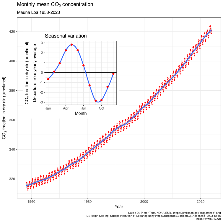
The Keeling curve. Charles David Keeling began continuous CO₂ measurements at the Mauna Loa Observatory in Hawaii in 1958, when the level was about 315 ppm; NOAA and the Scripps Institution continue them. The observatory sits high on a remote volcano in the middle of the Pacific, so it samples well-mixed air. Three features are tested. (1) The rise: from about 315 ppm to about 424 ppm (2024), roughly 50% above the pre-industrial 280 ppm; its monthly mean first topped 400 ppm in 2014 and its annual mean in 2015. (2) The acceleration: growth averaged about 0.8 ppm per year in the 1960s and about 2.4 ppm per year in 2011 to 2020, with a record jump of about 3.5 ppm from 2023 to 2024 (strong El Niño plus fires). (3) The sawtooth: about 6 to 7 ppm peak-to-trough at Mauna Loa, maximum in May (after winter decay with little photosynthesis) and minimum in September or October (after the summer growing season). The cycle is larger at high northern stations such as Point Barrow, Alaska, and is only about 1 ppm at the South Pole, because most land vegetation is in the Northern Hemisphere. Ice cores extend the record: CO₂ stayed between about 180 ppm (glacial periods) and 300 ppm (warm interglacials) for the past 800,000 years.
Why CO₂ is more evenly mixed than methane: CO₂ and methane both last long enough to mix around the globe (mixing between hemispheres takes about a year), but sources are concentrated in the Northern Hemisphere, so both are higher in the north: CO₂ by under 1% (a few ppm), methane by roughly 5% (about 100 ppb). Short-lived gases such as NO₂ and SO₂ never mix and stay near their sources.
Air quality connections. The US EPA's six criteria air pollutants are ground-level ozone, particulate matter (PM2.5 and PM10), carbon monoxide, lead, sulfur dioxide and nitrogen dioxide; CO₂ is not one of them. PM2.5 means particles with aerodynamic diameter of 2.5 µm or less. Acid rain forms when SO₂ and NOₓ are oxidized to sulfuric acid (H₂SO₄) and nitric acid (HNO₃); natural rain is already slightly acidic (pH about 5.6) from dissolved CO₂, and acid rain is typically pH 4.2 to 4.4.
Water vapor has no defined GWP: it stays in the air only about 9 days and its amount is controlled by temperature, so it acts as a feedback, not a forcing agent. In a ranking of GWP, water vapor goes last: H₂O < CO₂ (1) < CH₄ < N₂O < CFCs and HFCs < SF₆.
Methane sources in the United States. In the EPA's greenhouse-gas inventory, the largest human methane sources are oil and natural gas systems (leaks and venting from wells, pipelines and processing, together roughly a third), enteric fermentation in cattle and other livestock (roughly a quarter to 30%), landfills (roughly 15 to 20%), manure management (about 10%) and coal mining (about 6%). Globally, agriculture (livestock and rice) is the largest human source, followed by fossil fuels and waste.
GWP fine print. Methane's GWP-20 is about 84 in the IPCC's AR5 (86 including climate-carbon feedbacks) and about 81 in AR6 (about 80 for non-fossil and 83 for fossil methane); many keys use 84 to 86. Tropospheric ozone has no standard GWP: it is not emitted but formed from NOx, CO, VOCs and methane, and lasts only weeks, so its warming is credited to those precursors; if a ranking includes it anyway, the order is CO₂ < CH₄ < tropospheric O₃ < CFCs. Agriculture's direct greenhouse emissions are mainly CH₄ (livestock digestion, manure, rice paddies) and N₂O (fertilized soils); its CO₂ comes mostly from land clearing and fuel, which inventories count separately. When a water molecule absorbs an infrared photon it vibrates and rotates faster; the energy is re-emitted as infrared or shared with neighboring molecules as heat.
Ozone: shield above, pollutant below
About 90% of atmospheric ozone is in the stratosphere, concentrated between about 15 and 35 km (the ozone layer). The rest is in the troposphere. The same molecule plays opposite roles in the two places.
Stratospheric ozone forms and is destroyed by sunlight in the Chapman cycle:
- (photolysis of oxygen)
- (M is any third molecule that carries away energy)
- (ozone absorbs UV and is split, warming the stratosphere)
- (loss)
Reaction 3 is the shield. Ozone absorbs ultraviolet strongly in the Hartley band (about 200 to 310 nm) and more weakly in the Huggins bands (about 310 to 360 nm), and absorbs weakly in the visible Chappuis band (about 400 to 650 nm, peaking near 600 nm, with a weak tail to about 850 nm); it also has an infrared band at 9.6 µm, which makes it a greenhouse gas. Absorbed UV heats the stratosphere, which is why temperature increases with height there (a temperature inversion that suppresses vertical mixing).
| UV band | Wavelength | What ozone and air do to it |
|---|---|---|
| UV-C | 100 to 280 nm | Completely absorbed by O₂ and O₃; none reaches the ground |
| UV-B | 280 to 315 nm | Mostly absorbed by ozone; the part that gets through causes sunburn and skin cancer, so ozone loss raises surface UV-B |
| UV-A | 315 to 400 nm | Mostly transmitted; most UV reaching the ground |
Total ozone is measured in Dobson units (DU): 1 DU is a layer of pure ozone 0.01 mm thick at 0 °C and 1 atmosphere. The global average is about 300 DU, so all the ozone overhead would make a layer only about 3 mm thick. Ozone is made mostly over the tropics but carried poleward and downward by the slow Brewer-Dobson circulation, so totals are highest at middle and high latitudes in late winter and spring.
Catalytic destruction. Chlorine and bromine atoms released when UV breaks up CFCs and halons in the stratosphere destroy ozone without being used up: , then , net . One chlorine atom can destroy tens of thousands of ozone molecules before it is locked up. Most stratospheric chlorine is normally stored in harmless reservoir molecules, hydrogen chloride (HCl, formed when Cl reacts with methane) and chlorine nitrate (ClONO₂). Bromine (from halons and methyl bromide) is far more destructive per atom. N₂O is the main natural source of the nitrogen oxides that destroy ozone in the middle stratosphere, and is now the largest remaining emission of an ozone-depleting substance. The ozone depletion potential (ODP) of a substance compares its ozone destruction with that of the same mass of CFC-11, whose ODP is 1 by definition; HFCs have ODP 0.

The Antarctic ozone hole is the area where total ozone falls below 220 DU. It was reported by British Antarctic Survey scientists in 1985 and appears every southern spring, deepening in September and reaching its largest area in late September or early October, then filling in by December. The sequence:
- In the polar winter darkness, a strong polar vortex of westerly winds isolates the air over Antarctica, and it becomes extremely cold.
- Below about −78 °C, polar stratospheric clouds (PSCs) of nitric acid and ice form.
- On the cloud particles, the reservoirs react: . The nitric acid stays in the particles, which can fall out (denitrification), so chlorine cannot be locked back up.
- When sunlight returns in spring, it splits Cl₂ into free chlorine atoms, which destroy ozone rapidly through the ClO dimer cycle.
- As the stratosphere warms and the vortex breaks up in late spring, ozone-rich air mixes back in.
The Arctic has smaller, irregular losses because its stratosphere is warmer and its vortex weaker and more disturbed; warmer winters mean fewer PSCs and less destruction. Aura's MLS showed the inverse relationship directly: where ClO is high, ozone is low.
Policy. The Montreal Protocol (signed 1987, in force 1989, ratified by every UN member) phased out CFCs, halons and other ozone-depleting substances; HCFCs are being phased out as transitional replacements. Stratospheric chlorine peaked around the late 1990s and is declining, and the ozone layer is projected to return to 1980 levels around 2040 globally, about 2045 in the Arctic and about 2066 over Antarctica (2022 WMO/UNEP assessment). Because CFCs are also strong greenhouse gases, Montreal has done more to slow warming than any climate treaty. The Kigali Amendment (agreed 2016, in force 2019) adds a phase-down of HFCs, the ozone-safe but high-GWP replacements; ways to reduce HFC emissions include switching to low-GWP refrigerants (ammonia, CO₂, hydrocarbons, HFOs), fixing leaks and recovering refrigerant from old equipment. HFC concentrations and emissions rose quickly from the 1990s because HFCs replaced CFCs and HCFCs in refrigerators, air conditioners, foams and aerosol cans; HFC-134a is the most abundant. In the United States, the AIM Act (2020) set an 85% HFC production and use phase-down by 2036, matching Kigali. Global HFC emissions are still rising, but more slowly, as the phase-down starts.
Ozone and temperature. Ozone loss cools the stratosphere (less UV absorbed) and is a small negative forcing at the surface. Rising CO₂ also cools the stratosphere, because in the thin upper air extra CO₂ radiates more energy to space than it absorbs from below. A warming troposphere under a cooling stratosphere is a fingerprint of greenhouse forcing: a brighter Sun would warm both layers.
Ground-level ozone is a secondary pollutant: it is not emitted but forms when sunlight splits NO₂ (, then ) and volatile organic compounds (VOCs) keep converting NO back to NO₂ without using up ozone, so ozone builds up. It peaks on hot, sunny, stagnant summer afternoons downwind of cities. It is the main ingredient of photochemical smog, damages lungs and crops, and is a greenhouse gas (positive forcing).
Total ozone also has a seasonal cycle outside the ozone hole. It is set by sunlight, which changes with Earth's axial tilt and the Sun's angle, together with the Brewer-Dobson circulation that carries ozone from the tropical stratosphere, where most is made, toward the poles in winter and spring. Mid- and high-latitude totals therefore peak in late winter and spring and are lowest in autumn. CFCs were invented in 1928 by Thomas Midgley Jr. (for General Motors' Frigidaire division) as non-toxic, non-flammable refrigerants to replace ammonia, sulfur dioxide and methyl chloride, and were later used in aerosol sprays, foam blowing and solvents.
Aerosols
An aerosol is a suspension of fine solid particles or liquid droplets in a gas; in climate science the word usually means the particles themselves (about 0.01 to 10 µm). SO₂ is a gas, not an aerosol, until it is oxidized to sulfate particles.
Aerosols also affect rainfall. By reflecting and absorbing sunlight they dim the surface (surface dimming), which reduces evaporation and the energy that drives convection, so a heavily polluted region can get less rain. Northern Hemisphere sulfate pollution in the twentieth century cooled that hemisphere and is thought to have pushed the tropical rain belt (ITCZ) south, contributing to the Sahel drought of the 1970s and 1980s. Dust from desertified land then adds more aerosol, a feedback that can sustain drought.
| Aerosol | Natural sources | Human sources | Main radiative effect |
|---|---|---|---|
| Sea salt | Sea spray from breaking waves (the largest source by mass) | — | Scatters, cools; good cloud condensation nuclei |
| Mineral dust | Deserts (Sahara, Gobi), dust storms | Disturbed soils, agriculture, drying lakes | Scatters and somewhat absorbs; mixed sign |
| Sulfate | Volcanoes; dimethyl sulfide (DMS) from plankton | Coal and oil burning, smelting, shipping | Strongly scatters (single-scattering albedo near 1), cools; brightens clouds |
| Nitrate and ammonium | Lightning, soils | Vehicles, power plants, fertilizer and livestock (NH₃) | Scatters, cools |
| Black carbon (soot) | Wildfires | Diesel engines, coal, cookstoves, crop burning | Absorbs sunlight, warms the air; darkens snow and ice when deposited |
| Organic carbon, smoke | Wildfires, forest emissions (secondary organic aerosol from isoprene and terpenes) | Biomass burning, fossil fuels | Mostly scatters; "brown carbon" absorbs in the UV |
| Volcanic ash | Explosive eruptions | — | Falls out in days to weeks; the long-lived effect comes from sulfate |
Aerosols are short-lived in the lower atmosphere (about a week before rain removes them), so unlike CO₂ they are concentrated near their sources and downwind: their forcing is patchy, strongest over and downwind of industrial and burning regions, and much larger in the Northern Hemisphere. In the stratosphere, where there is no rain, volcanic sulfate lasts one to two years, which is why only eruptions that reach the stratosphere change global climate.
How aerosols change the energy budget:
- Direct effect (aerosol-radiation interaction): particles scatter sunlight back to space (cooling) or absorb it (warming the air layer, cooling the surface beneath). The balance depends on the single-scattering albedo (SSA), the fraction of extinction that is scattering rather than absorption: about 1 for sulfate, about 0.8 to 0.95 for smoke, and much lower for pure black carbon. It also depends on the aerosol optical depth (how much there is), on the brightness of what is underneath (an absorbing layer over a dark ocean cools at the top of the atmosphere but over a bright cloud or snow warms) and on the layer height (absorbing aerosol above clouds warms most).
- Indirect effects (aerosol-cloud interaction): aerosols are cloud condensation nuclei (CCN, typically about 0.1 to 1 µm). The Twomey effect: more CCN spread the same water over more, smaller droplets, which have more total surface area, so the cloud's optical depth and albedo rise and it cools more. The Albrecht (lifetime) effect: smaller droplets collide and merge less efficiently, so drizzle is suppressed and clouds last longer and cover more area, cooling further. Ship tracks, bright lines in low clouds behind ships, are the visible example.
- Semi-direct effect: absorbing black carbon heats the cloud layer and can evaporate clouds, a warming effect.
Overall, IPCC AR6 assesses human aerosols' effective radiative forcing at about −1.1 W/m² (1750 to 2019), masking roughly a third of greenhouse-gas forcing. Reducing sulfur emissions for health reasons therefore unmasks warming: the 2020 International Maritime Organization rule that cut the sulfur limit in ship fuel from 3.5% to 0.5% reduced ship tracks and is estimated to have added a small positive forcing. Statements such as "the 40% drop in SO₂ emissions has cooled the planet" are false. This aerosol masking, and the dimming of sunlight at the surface it caused in the mid-20th century, is called global dimming.
Examples that tests use: Mount Pinatubo (Philippines, June 1991) injected about 15 to 20 million tonnes of SO₂ into the stratosphere, and global temperature fell by roughly 0.5 °C in 1992; Tambora (Indonesia, 1815) caused the "Year Without a Summer" in 1816. A CALIPSO curtain months after an eruption shows a thin, high layer in the stratosphere. Stratospheric aerosol injection, a proposed geoengineering method, would imitate this: it would cool the troposphere and surface but warm the stratosphere, where the sulfate absorbs infrared and near-infrared. The CLAW hypothesis (1987) proposed a negative feedback: warmer, sunnier oceans grow more phytoplankton, which release DMS; DMS forms sulfate CCN; more CCN brighten marine clouds and cool the surface.
The direct radiative forcing of an aerosol at the top of the atmosphere is the change in net downward flux it causes: for sunlight, the reflected (upward) flux without aerosol minus the reflected flux with it. Computed for clear sky it is usually negative (cooling); computed with clouds present it is smaller, and it turns positive (warming) when absorbing smoke or soot lies above bright cloud, because the aerosol darkens a bright scene. Marine cloud brightening is a proposed geoengineering method that sprays sea-salt particles into low marine clouds to exploit the Twomey effect, making them brighter (higher albedo) to cool the surface; stratospheric aerosol injection would mimic a volcanic eruption instead.
Absorbing aerosols also change circulation. Dust and black carbon absorb sunlight and warm the layer they sit in (diabatic heating) while dimming the surface. Over South Asia, absorbing aerosol piled against the Himalayas and Tibetan Plateau in spring heats the air aloft, which draws in moist air and can strengthen and advance the early monsoon rains (the "elevated heat pump" hypothesis), even though the dimmed surface weakens convection later.
Separating dust with lidar. Lidar uses two numbers. The depolarization ratio is near zero for spherical particles (cloud droplets, sulfate, most smoke: below about 0.05 to 0.1) and high for irregular particles (dust about 0.3; ice crystals higher). The lidar ratio (extinction-to-backscatter, in sr) is about 40 to 55 sr for dust, about 20 sr for sea salt and about 50 to 80 sr for smoke and pollution. CALIPSO's algorithm uses depolarization to flag dust, and research retrievals use it to split a mixed layer's extinction into dust and non-dust parts.
Aerosols and clouds in more detail. Many small cloud-condensation nuclei make many small droplets that are slow to collide and rain out, so warm rain is suppressed and more water is carried above the freezing level; when it freezes it releases extra latent heat, which can invigorate deep convection, giving fewer but heavier downpours (the invigoration hypothesis). The Southern Ocean shows the clean extreme: it has few, mostly natural nuclei (sea salt and sulfate from phytoplankton DMS), so its clouds have fewer, larger droplets, lower albedo and more drizzle than polluted Northern Hemisphere clouds, plus abundant supercooled liquid water. Cloud seeding for rain or snow uses silver iodide (sometimes dry ice or salt) as artificial nuclei.
Aerosol optical depth and visibility are linked: AOD below about 0.1 means very clear air (visibility tens of kilometers or more), about 0.3 to 0.5 noticeable haze, above about 1 thick smoke or dust, and values of 3 to 5 or more occur in dense wildfire smoke or dust storms, when visibility falls to about a kilometer or less.
Clouds and their radiative effects
At any time about two-thirds of Earth is covered by cloud. Clouds are named by height and form.
| Level | Typical base height (mid-latitudes) | Types | Made of | Radiative character |
|---|---|---|---|---|
| High | Above about 6 km (about 5 to 13 km; higher in the tropics) | Cirrus, cirrostratus, cirrocumulus; contrails | Ice crystals | Thin and cold: let most sunlight through but trap outgoing infrared, so they warm |
| Middle | About 2 to 7 km | Altostratus, altocumulus | Water, ice or both | Intermediate |
| Low | Below about 2 km | Stratus, stratocumulus, nimbostratus (thick rain layer) | Water droplets | Thick and bright but warm-topped: reflect much sunlight and emit almost as much infrared as the surface, so they cool |
| Vertical | Base low, top up to the tropopause (12 to 18 km) | Cumulus, cumulonimbus | Water below, ice above | Very high albedo (up to about 0.9) and very cold tops: large cooling and warming terms that nearly cancel |
The mechanism behind the cooling-versus-warming split is two numbers: the cloud's albedo, which rises with thickness, liquid water and smaller droplets, and its top temperature, which falls with height. A low cloud has a high albedo and a warm top, so it reflects a lot of sunlight but barely reduces outgoing longwave (stratocumulus decks over cool subtropical oceans are the strongest cooling clouds on Earth). A high thin cirrus has a low albedo but a cold top, so it emits much less infrared to space than the warm surface below would have, a net warming. Cirrus and contrails, made by aircraft exhaust water vapor freezing in cold, humid air, are the best-known warming clouds.
The cloud radiative effect (CRE, also called cloud forcing) is the difference between all-sky and clear-sky top-of-atmosphere flux. CERES measures it globally at about −45 to −47 W/m² in the shortwave (cooling by reflection) and about +26 to +28 W/m² in the longwave (warming by trapping), a net of about −20 W/m²: clouds as a whole cool the planet. Clouds reflect about 20 to 23% of incoming sunlight, about two-thirds of Earth's total albedo of about 0.30. Clouds also narrow the daily temperature range: cloudy days are cooler (less sunlight in) and cloudy nights warmer (more infrared returned), so a sky cloudy both day and night gives the smallest range.
Cloud feedback asks how clouds change as the planet warms. AR6 assesses it as positive (amplifying), about +0.4 W/m² per K, with the largest uncertainty of any feedback: high clouds rise and their tops stay cold while the surface warms (positive), low clouds over the subtropical oceans thin and shrink (positive), while clouds at high latitudes contain more liquid and become brighter (negative). Higher humidity over oceans and the large contrast between dark ocean and bright cloud make the shortwave cloud effect larger over oceans than over land.
Cloud names are built from Latin roots: cirro- (curl or wisp of hair: high ice clouds), strato- (layer or sheet), cumulo- (heap or pile), nimbo-/-nimbus (rain-bearing) and alto- (middle level, despite meaning "high"). So nimbostratus is a rain-bearing layer and cumulonimbus a rain-bearing heap.
Nearly all clouds and weather are in the troposphere. The exceptions are polar stratospheric clouds (in the winter polar stratosphere, about 15 to 25 km, which drive ozone-hole chemistry) and noctilucent (polar mesospheric) clouds of ice near 80 to 85 km in the summer polar mesosphere.
Climate drivers and circulation
A climate forcing is an imposed change in Earth's energy budget from outside the climate system's own internal dynamics: changes in the Sun, Earth's orbit, volcanic aerosols, greenhouse gases, human aerosols and land-surface albedo. Internal variability, such as ENSO and the North Atlantic Oscillation, moves energy around within the system without an outside cause. The climate system has five components: atmosphere, hydrosphere (oceans, lakes, rivers, groundwater), cryosphere (all frozen water: sea ice, glaciers, ice sheets, snow cover, lake and river ice, and permafrost; it matters because ice and snow have high albedo and store fresh water), lithosphere (land surface) and biosphere. Weather is the state of the atmosphere at a given time and place; climate is the long-term statistics (usually 30-year averages) of weather. An anomaly is the departure from the average for the same place and time of year.
Internal or external? External forcings: solar variability, Milankovitch orbital cycles (which pace the ice ages, so glacial-interglacial cycles count as externally forced, amplified by internal CO₂ and ice-albedo feedbacks), volcanic eruptions, and human greenhouse gases, aerosols and land-use change. Internal variability: ENSO, the North Atlantic Oscillation, the Pacific Decadal Oscillation, monsoon variability and weather noise. A La Niña year is cooler because of internal variability, not a negative forcing.
Climate models and parameterization. Global climate models divide the atmosphere and ocean into grid cells tens to hundreds of kilometers wide and step the equations of fluid motion, energy and moisture forward in time. Processes smaller than a grid cell (individual clouds and convection, turbulence, radiation details, aerosol-cloud interactions) cannot be resolved, so they are parameterized: represented by simplified formulas tied to grid-scale variables. Cloud and convection parameterizations are the largest source of spread among models' climate sensitivity, which is why satellite cloud data (CloudSat, CALIPSO, MODIS, CERES) are used to test models.
| Driver | Timescale | Size | How it works |
|---|---|---|---|
| Solar cycle | About 11 years (sunspot cycle) | Total solar irradiance varies about 0.1% (about 1 W/m² of 1,361), so about 0.2 W/m² of absorbed forcing | More sunspots coincide with a slightly brighter Sun (faculae outweigh the dark spots); UV varies much more than visible light, so the upper atmosphere responds most (the thermosphere heats and expands). The Maunder Minimum (about 1645 to 1715) had almost no sunspots. Solar changes cannot explain recent warming: irradiance has been flat or slightly falling since the 1980s while temperature rose |
| Volcanic eruptions | 1 to 3 years per eruption | Up to several W/m² negative for a large eruption | Stratospheric sulfate reflects sunlight; volcanic CO₂ is only about 1% of human emissions |
| Milankovitch cycles | Tens to hundreds of thousands of years | Small change in global annual sunlight but large changes by season and latitude | Orbital changes pace the ice ages; feedbacks (ice albedo, CO₂) amplify them |
| Greenhouse gases | Decades to millennia | About +3.3 W/m² from all well-mixed GHGs since 1750 | Absorb outgoing infrared |
| Aerosols and land use | Days (aerosols) to decades | About −1.1 W/m² (aerosols) and −0.2 W/m² (land albedo) | Reflect sunlight; brighten clouds; deforestation raises albedo |
| Plate tectonics and weathering | Millions of years | Large | Move continents, build mountains, control CO₂ through volcanic outgassing and rock weathering |
Milankovitch cycles are the periodic changes in Earth's orbit and axis, named for Milutin Milanković.
| Cycle | What changes | Range | Period |
|---|---|---|---|
| Eccentricity | How elliptical the orbit is | About 0.0 to 0.06; now 0.0167 | About 100,000 years, and about 405,000 years |
| Obliquity (axial tilt) | Angle of the axis to the orbit's perpendicular | 22.1° to 24.5°; now 23.44° and decreasing | About 41,000 years |
| Precession | Which season occurs at perihelion (axial precession plus the slow turning of the orbit) | Perihelion now falls in early January, during northern winter | Axial precession about 26,000 years; the climatic precession cycle about 19,000 to 23,000 years |
Larger tilt means hotter summers and colder winters at high latitudes. Ice ages begin when northern summers are cool enough for winter snow to survive (low tilt, Northern summer at aphelion); feedbacks from ice albedo and from CO₂ released or absorbed by the ocean amplify the small orbital push. The last 800,000 years have had glacial cycles about 100,000 years long.
Seasons come from the 23.44° tilt, not from distance to the Sun: Earth is actually closest to the Sun (about 147 million km) in early January and farthest (about 152 million km) in early July, which changes the solar constant by only about 7%. Tilt changes both the angle of sunlight (low Sun spreads the same beam over more ground and through a longer path of air) and the length of day. That is also why the tropics receive more energy than the poles: flux on a horizontal surface is , where is the solar zenith angle. The Southern Hemisphere has the lowest albedo in its summer, when snow cover is least and sea ice smallest.
Atmospheric circulation carries heat from the tropical energy surplus toward the poles.
- Hadley cells (equator to about 30°): air rises at the intertropical convergence zone (ITCZ), where the trade winds meet and rain is heaviest; it flows poleward aloft, sinks around 30° (the subtropical highs, where most great deserts lie) and returns as the easterly trade winds.
- Ferrel cells (about 30° to 60°): surface westerlies; the mid-latitude storm track.
- Polar cells (about 60° to 90°): cold air sinks at the pole and spreads out as polar easterlies.
- Jet streams are fast westerly winds near the tropopause: the polar jet (about 50° to 60°, strongest where the temperature contrast between polar and mid-latitude air is sharpest) and the subtropical jet (about 30°). A weaker, wavier polar jet lets weather systems stall, producing long heat waves under blocking highs and cold outbreaks further south.
- Monsoons are seasonal wind reversals driven by land heating faster than ocean in summer.
- High-pressure systems have sinking air and weak winds, which suppress vertical mixing and trap pollutants near the ground.
Ocean circulation carries the rest of the poleward heat. Wind-driven gyres circulate around each ocean basin, with fast warm western boundary currents such as the Gulf Stream. Winds blowing along the eastern edges of the oceans drive coastal upwelling (off Peru, California, northwest and southwest Africa), bringing cold, nutrient-rich water up and supporting rich fisheries. The thermohaline circulation, driven by differences in temperature and salinity, sinks cold, salty water in the North Atlantic (the Nordic and Labrador Seas) and around Antarctica and spreads it through the deep ocean over about a thousand years. Its Atlantic branch, the Atlantic Meridional Overturning Circulation (AMOC), warms northwestern Europe; meltwater and warming make the surface water lighter, which is expected to weaken it. The ocean is the largest heat buffer in the climate system: it has absorbed about 90% of the extra energy from the energy imbalance.
Polar amplification: the Arctic has warmed about three to four times as fast as the global average since 1979, because of ice-albedo feedback, a lapse-rate feedback that is positive at high latitudes (warming is trapped near the surface in the stable polar air) and heat carried poleward. The faint young Sun paradox: the Sun was about 25 to 30% dimmer about 4 billion years ago, yet geology shows liquid water on early Earth, which requires a much stronger greenhouse effect (more CO₂, and perhaps methane) or a lower albedo then.
A short history of greenhouse science. Joseph Fourier (1820s) argued that the atmosphere keeps Earth warmer than sunlight alone would. Eunice Foote (1856) showed that air with CO₂ warmed more in sunlight, and John Tyndall (1859) measured the infrared absorption of water vapor and CO₂. Svante Arrhenius (1896) made the first calculation linking CO₂ to temperature, estimating several degrees of warming for a doubling. Guy Callendar (1938) connected rising CO₂ from fossil fuels to observed warming, and Charles Keeling began the Mauna Loa record in 1958.
Climate change effects on weather and ecosystems
Global mean surface temperature (GMST) is the area-weighted average of near-surface air temperature over land and sea-surface temperature over the oceans, reported as an anomaly from a baseline. IPCC AR6 measured 2011 to 2020 at about 1.1 °C above 1850 to 1900; 2024 was the warmest year on record at about 1.55 °C above that baseline (WMO), the first calendar year above 1.5 °C. Climate change is broader than global warming: it includes changes in precipitation, extremes, sea level and ice.
| Change | Mechanism | Remote-sensing evidence |
|---|---|---|
| Heavier downpours and flooding | Clausius-Clapeyron: saturation vapor pressure rises about 7% per °C, so warmer air holds and delivers more water when it rains, even where total rainfall declines | GPM rain rates; Sentinel-1 and MODIS flood maps |
| More intense droughts | Higher evaporative demand dries soils; shifted storm tracks | GRACE water storage loss; ECOSTRESS stress; NDVI decline |
| Heat waves | Warmer baseline; dry soils cannot cool by evaporation; stalled high-pressure systems | MODIS, ECOSTRESS land surface temperature |
| Heat domes | A stalled ridge of high pressure with sinking, warming air | Persistent clear skies and record land surface temperature in MODIS, GOES and ECOSTRESS |
| Atmospheric rivers | Warmer air carries more vapor (Clausius-Clapeyron) | Long, narrow plumes in GOES water-vapor imagery and microwave total-precipitable-water maps; GPM rain totals |
| Wildfires and smoke | Longer fire seasons, drier fuels, more lightning; most severe increase in boreal forests of North America and Siberia | GOES and MODIS fire detection (thermal hot spots), AOD, TROPOMI CO; smoke cools the surface under it but absorbing smoke warms the air above, and greenhouse gases released add long-term warming |
| Stronger tropical cyclones | Warmer oceans; more moisture; higher seas raise storm surge | A larger share of storms reach the highest categories and rain rates rise; the total number is not clearly increasing |
| Sea-ice loss | Warming and ice-albedo feedback | Arctic September minimum extent declining about 12 to 13% per decade since 1979 (passive microwave) |
| Glacier and ice-sheet loss | Warming air and ocean | GRACE mass loss; ICESat-2 heights; Landsat retreat |
| Permafrost thaw | Warming soils | InSAR ground subsidence, lake changes; hard to see the subsurface directly |
| Biome shifts | Species move toward the poles and upslope; boreal forest advances into tundra; treelines rise, compressing alpine habitats | NDVI and EVI trends: "Arctic greening" from longer growing seasons |
| Earlier spring (phenology) | Warmer springs | Earlier NDVI green-up dates |
| Coral bleaching | Water about 1 °C above the usual summer maximum makes corals expel their symbiotic algae (zooxanthellae); acidification weakens their skeletons | SST anomalies and NOAA Coral Reef Watch "degree heating weeks" |
A biome shift of boreal forest into tundra is a positive feedback: the dark canopy sticking out above snow has a much lower albedo than snow-covered tundra, so the region absorbs more sunlight and warms further. Species most likely to survive have wide climatic tolerance ranges. CO₂ fertilization has made the planet greener overall, but heat and drought stress can turn forests from carbon sinks into carbon sources: a forest that releases more carbon than it absorbs is a carbon source.
Tipping points are thresholds beyond which a part of the climate system changes self-sustainingly and is hard to reverse. The 2025 Global Tipping Points Report concluded that warm-water coral reefs have already passed theirs (estimated near 1.2 °C of warming). The Greenland and West Antarctic ice sheets, permafrost and the North Atlantic subpolar gyre have estimated thresholds around 1.5 °C, close to current warming, and the Amazon rainforest (whose threshold deforestation may be lowering) and AMOC have higher, more uncertain central estimates. If a test asks which element is closest to or already past its threshold, coral reefs and then the Greenland and West Antarctic ice sheets are the expected answers.
Forests as carbon sinks. Boreal and temperate forests remain net carbon sinks, but intact tropical forests have weakened as sinks; with deforestation, fire and degradation the tropics as a whole are now roughly carbon-neutral or a net source in some estimates (parts of the southeastern Amazon emit more than they absorb). Hotter, drier conditions are expected to reduce local tree species richness as narrow-tolerance species decline or shift.
Coral bleaching. NOAA Coral Reef Watch flags thermal stress when sea-surface temperature exceeds the long-term maximum monthly mean by about 1 °C. Accumulated stress is measured in degree heating weeks (DHW, °C-weeks above that threshold over 12 weeks): about 4 DHW brings significant bleaching and about 8 DHW severe, widespread bleaching and mortality. For many tropical reefs the danger zone begins near 29 to 30 °C.
Photosynthesis pathways. Most plants (wheat, rice, trees) use C3 photosynthesis, which loses efficiency in heat because the enzyme RuBisCO increasingly grabs O₂ instead of CO₂ (photorespiration). C4 plants (corn, sugarcane, many tropical grasses) concentrate CO₂ around RuBisCO, so they do better in hot, sunny, drier climates. CAM plants (cacti, pineapple, agave) open their stomata only at night to save water, suiting deserts. Rising CO₂ benefits C3 plants most; rising heat and drought favor C4 and CAM plants.
El Niño–Southern Oscillation
The El Niño–Southern Oscillation (ENSO) is a coupled ocean-atmosphere cycle in the tropical Pacific. Normally, trade winds blow west along the equator, piling warm surface water in the west, deepening the warm layer there and letting cold, nutrient-rich water well up along South America. During El Niño, the trade winds weaken, warm water spreads east, upwelling along South America is suppressed, and the sea surface in the east becomes higher as well as warmer. During La Niña, the trade winds strengthen, the east cools further and upwelling increases.
Regional effects are the most tested part; they are tabulated in "ENSO impacts by region" below. In satellite questions, look for sea-surface temperature anomalies in the equatorial eastern Pacific (MODIS on Aqua, GOES) or sea-surface-height anomalies (JASON) to identify the phase.
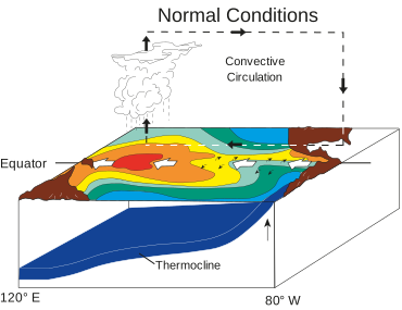

The machinery. The Walker circulation is the east-west loop over the equatorial Pacific: air rises over the warm western Pacific (heavy rain over Indonesia), flows east aloft, sinks over the cool eastern Pacific (dry coastal Peru and Chile) and returns west as the trade winds. The thermocline, the boundary between warm surface water and cold deep water, normally tilts: deep (about 150 to 200 m) in the west and shallow (tens of meters) in the east, and sea level is roughly half a meter higher in the west than in the east. The Bjerknes feedback couples these: a warmer east weakens the east-west temperature contrast, which weakens the trade winds, which lets more warm water slosh east and deepens the eastern thermocline, which warms the east further. That positive feedback grows an El Niño (or, run the other way, a La Niña). Negative feedbacks end events: the ocean adjusts through slow Kelvin waves (eastward-moving bulges of warm water and a deepened thermocline along the equator, visible in Jason sea-surface height as a +5 to +20 cm ridge traveling east over about two months) and reflected Rossby waves, so each event eventually reverses. ENSO recurs irregularly every 2 to 7 years; events usually peak in northern winter and last about 9 to 12 months, La Niña sometimes longer. Between events conditions are ENSO-neutral.
How it is measured.
- Oceanic Niño Index (ONI): NOAA's official index, the 3-month running mean of SST anomalies in the Niño 3.4 region (5° N to 5° S, 120° W to 170° W). El Niño conditions: ONI ≥ +0.5 °C; La Niña: ≤ −0.5 °C; an episode is declared when the threshold holds for at least five consecutive overlapping 3-month seasons. Strength categories are often quoted as weak (0.5 to 0.9), moderate (1.0 to 1.4), strong (1.5 to 1.9) and very strong (2.0 or more).
- Southern Oscillation Index (SOI): the standardized difference in sea-level pressure between Tahiti (central Pacific) and Darwin, Australia (west). Normally Tahiti's pressure is higher; a sustained negative SOI (lower pressure at Tahiti, higher at Darwin) means El Niño, positive means La Niña. The "Southern Oscillation" is this atmospheric pressure seesaw.
- Satellites: SST anomaly maps (MODIS on Aqua for long consistent records from a sun-synchronous orbit; GOES for continuous coverage of the eastern Pacific) show a tongue of warm anomalies along the equator in the east during El Niño, cold during La Niña. Jason sea-surface-height anomaly maps show the same pattern as height: warmer water has expanded and the thermocline is deeper, so sea level is higher in the east (and lower in the west) during El Niño. TOPEX/Poseidon's tracking of the 1997 to 1998 El Niño made it famous. OLR and GPM rain maps show convection shifted into the central and eastern Pacific. OCO-2 and the Keeling curve show CO₂ growing faster during and after El Niño.
ReferenceENSO impacts by region· 14 rows
Typical patterns; any one event can differ. Winter means northern winter (December to February) unless stated.
No rows match.
| Region | El Niño | La Niña |
|---|---|---|
| Coastal Peru and Ecuador | Heavy rain and floods; warm water ends upwelling, collapsing anchovy fisheries and seabird colonies | Cooler, drier; strong upwelling and productive fisheries |
| Central and eastern tropical Pacific | Warmer SST, more rain and convection, higher sea level | Cooler SST, drier, lower sea level |
| Indonesia, Papua New Guinea, Philippines | Drought, peat and forest fires, haze | Wetter than normal, flooding |
| Eastern Australia | Drought, heat, bushfire risk; rainforests can switch from carbon sink to source | Wet, cool, flooding |
| India and South Asia | Weaker summer monsoon, drought risk | Stronger monsoon |
| Southern Africa | Drought in the summer rainy season | Wetter |
| East Africa | Wetter short rains (October to December) | Drier, drought |
| Northern South America (Colombia, Venezuela, northern Brazil) | Drought | Wetter |
| Southern United States and Gulf Coast | Cooler and wetter winter, more storms (subtropical jet strengthened and shifted south) | Warmer and drier winter, drought and fire risk |
| Pacific Northwest, northern Plains, Ohio Valley, Canada | Warmer, drier winter | Colder, wetter (snowier) winter |
| Atlantic hurricanes | Suppressed by stronger vertical wind shear | Enhanced (weaker shear) |
| Central and eastern Pacific hurricanes | Enhanced | Suppressed |
| Global mean temperature | Rises, by about 0.1 to 0.2 °C, peaking a few months after the event; El Niño years (1998, 2016, 2023 to 2024) set records | Falls slightly |
| Atmospheric CO₂ growth | Faster: tropical drought and fires weaken the land sink | Slower |
Is ENSO a forcing? No. ENSO is internal variability: it redistributes heat between the ocean and atmosphere rather than changing the energy entering or leaving the planet. A volcanic eruption cools by changing albedo (an external forcing); El Niño warms the surface by releasing ocean heat. Some test keys still label La Niña a "negative forcing (cooling)": if forced to choose, give the direction of its surface effect, but note that it is internal variability. If a strong El Niño coincides with a large eruption, the effects partly cancel: the global surface warms less than El Niño alone would make it.
ENSO and climate change. Warming adds to every ENSO state: El Niño years are the record years. Because a warmer atmosphere holds more water vapor, rainfall anomalies during events are expected to intensify; whether events will become more frequent or stronger is still uncertain.
Teleconnections. ENSO changes weather far from the Pacific through teleconnections: the shift of tropical rainfall and heating alters the large-scale atmospheric circulation (the Walker and Hadley circulations and the waves they send into the midlatitudes), which bends the jet streams and storm tracks. That is how a warm eastern Pacific can bring a wet winter to the southern United States, a mild winter to Canada, drought to southern Africa and fewer Atlantic hurricanes.
Carbon and nitrogen cycles
The carbon cycle moves carbon among the atmosphere, oceans, plants and soils. Photosynthesis takes CO₂ out of the air; respiration, decomposition and fire return it. Fossil-fuel burning and land-use change add carbon faster than natural sinks absorb it, and the ocean takes up part of the excess, which makes seawater more acidic. Remote sensing measures pieces of this: column CO₂ from OCO-2, vegetation greenness from optical sensors, and ocean chlorophyll (a proxy for marine primary production) from ocean-color sensors such as PACE and MODIS.
Primary production. Gross primary production (GPP) is the total carbon fixed by photosynthesis; net primary production (NPP) is GPP minus the carbon the plants themselves respire (autotrophic respiration), so it is the carbon stored as new plant growth, available to the rest of the ecosystem, usually in g C/m² per year. Land NPP is roughly 50 to 60 Gt C per year and ocean NPP about the same. From space, NPP is estimated with a light-use-efficiency model: absorbed photosynthetically active radiation (from NDVI or similar indices) times an efficiency reduced by temperature and water stress. MODIS produces global GPP and NPP products (MOD17), Landsat-based versions give 30 m detail for farms and forests, and ocean NPP comes from chlorophyll maps (MODIS, PACE). Net ecosystem production subtracts the respiration of animals and microbes too; a positive value means the ecosystem is a carbon sink.

Reservoirs. Carbon is measured in gigatonnes of carbon (GtC, g of carbon; multiply by 3.67 for the mass of CO₂). One ppm of atmospheric CO₂ is about 2.12 GtC.
| Reservoir | Approximate carbon (GtC) | Residence time | Notes |
|---|---|---|---|
| Sedimentary rocks (limestone and other carbonates, kerogen in shale) | Tens of millions | Hundreds of millions of years | By far the largest; part of the slow carbon cycle run by weathering, burial, subduction and volcanic outgassing |
| Deep ocean (dissolved inorganic carbon) | About 37,000 to 38,000 | About 1,000 years | Largest active reservoir |
| Fossil fuel reserves | About 1,000 to 2,000 (estimates vary) | Millions of years unless burned | Coal, oil, gas |
| Soils | About 1,500 to 2,400 (plus about 1,400 in permafrost) | Decades to millennia | More than plants and air combined |
| Surface ocean | About 900 | Years to a decade | Exchanges directly with the air |
| Atmosphere | About 900 in 2024 (about 590 pre-industrial) | A CO₂ molecule exchanges in about 4 to 5 years (older texts and keys say about 5 to 10 years), but an added excess persists for centuries | Rising about 5 GtC per year |
| Vegetation | About 450 to 650 | Years to centuries | Mostly in forest wood |
| Marine biota | About 3 | Days to weeks | Tiny stock but a large flux: phytoplankton fix about as much carbon each year as land plants |
Fluxes and the human perturbation. Natural exchanges are large and nearly balanced: land plants take up roughly 120 GtC per year by photosynthesis and release about the same by plant and soil respiration (the largest natural flux of carbon into the atmosphere) and fire; the ocean and atmosphere exchange about 80 to 90 GtC per year each way. Human emissions are smaller but one-directional. From 2014 to 2023 (Global Carbon Budget 2024), fossil fuels and cement released about 9.7 GtC per year and land-use change about 1.1 GtC per year, close to 11 GtC per year in total (about 40 Gt of CO₂). Of that, about 48% stayed in the atmosphere (the airborne fraction, about 5 GtC per year), about 26% went into the ocean and about 30% into the land biosphere, the land and ocean taking roughly equal shares (the shares add to slightly more than 100% because the Global Carbon Budget has an unexplained imbalance of a few percent). Both sinks are projected to absorb a smaller fraction as emissions continue, because warmer water dissolves less CO₂ and drought and heat stress plants. Since 1750, CO₂ has risen about 50%, methane about 166% and N₂O about 25%.
Each process moves carbon in one direction; decide whether it removes carbon from the air (sink) or adds it (source).
| Process | Carbon moves | Sink or source for the air? |
|---|---|---|
| Photosynthesis (land plants, phytoplankton): | Air → biomass | Sink |
| Respiration (plants, animals, microbes) | Biomass → air | Source |
| Decomposition (aerobic gives CO₂; anaerobic, in wetlands, landfills and rice paddies, gives CH₄) | Dead matter → air | Source |
| Combustion (fossil fuels, wildfire, burning a tree) | Fuel → air | Source |
| Ocean uptake (solubility pump) | Air → ocean | Sink |
| Biological pump: plankton fix carbon, some sinks as dead cells and fecal pellets to the deep sea | Surface → deep ocean and sediment | Sink |
| Carbonate formation (shells, coral, limestone) and peat or soil formation | Water or air → rock or soil | Long-term sink |
| Weathering of silicate rocks (uses CO₂ dissolved in rain) | Air → rivers → ocean sediments | Slow sink (thermostat over millions of years) |
| Volcanic and subduction outgassing | Rock → air | Slow source |
| Transpiration | Moves water, not carbon | Neither |
A carbon sink is any reservoir or process that takes up more carbon than it releases; a source releases more than it takes up. Ocean, forests, soils, peat and carbonate rocks are sinks. Blue carbon is carbon stored by coastal and marine ecosystems: mangroves, seagrass meadows and salt marshes. A burned or cleared forest becomes a source; heat waves increase respiration and reduce photosynthesis, giving a net release. Converting tropical forest to cropland releases CO₂ (burning, soil carbon loss) and raises N₂O (fertilizer, disturbed soils).
Ocean acidification. Dissolved CO₂ forms carbonic acid, which releases hydrogen ions:
The extra H⁺ lowers pH, and it combines with carbonate ions, so less carbonate (CO₃²⁻) is available to corals, shellfish, pteropods and coccolithophores that build calcium carbonate shells and skeletons. Surface ocean pH has fallen from about 8.2 before industrialization to about 8.1 now; because pH is logarithmic, a drop of 0.1 means about times as many hydrogen ions, an increase of about 26 to 30%. Satellites cannot measure pH directly; they monitor related quantities (SST, chlorophyll, coral reef condition) and ships, buoys and floats measure the chemistry. Warmer water holds less CO₂ (lower solubility) and a more stratified ocean mixes surface carbon down more slowly, both weakening the ocean sink, a positive feedback.
Nitrogen. The nitrogen cycle is linked through plant growth. Nitrogen-fixing bacteria (and lightning, and the industrial Haber-Bosch process for fertilizer) convert atmospheric N₂ into forms plants can use; microbes later return it as N₂ and as N₂O by denitrification. Excess fertilizer therefore raises N₂O emissions, and runoff feeds algal blooms that change ocean color. Combustion nitrogen oxides feed ozone and aerosol formation.
Nitrogen gas makes up 78% of the air, but its triple bond makes it unusable by almost all organisms. Converting N₂ into a reactive form is nitrogen fixation, and there are four main pathways:
| Fixation pathway | What happens |
|---|---|
| Biological fixation (the largest natural pathway) | Diazotrophs, bacteria and archaea with the enzyme nitrogenase, make ammonia: . Examples: Rhizobium in root nodules of legumes (soybeans, peas, clover, alfalfa), free-living Azotobacter, cyanobacteria in water and rice paddies, Frankia on alder trees |
| Lightning (atmospheric fixation) | The heat of a lightning bolt splits N₂ and O₂, forming nitrogen oxides that rain out as nitrate; the main source of NOₓ in the upper troposphere |
| Industrial Haber-Bosch process | at high temperature (about 400 to 500 °C) and pressure (about 150 to 300 atm) over an iron catalyst; makes synthetic fertilizer |
| Combustion | High-temperature burning in engines and power plants combines N₂ and O₂ into NOₓ |
The other steps move nitrogen that is already reactive; they are not fixation:
| Step | Conversion | Organisms and conditions |
|---|---|---|
| Assimilation | NH₄⁺ or NO₃⁻ taken up into amino acids and proteins | Plants, algae, microbes; animals get nitrogen by eating them |
| Ammonification (mineralization) | Organic nitrogen in dead matter and waste → NH₃ / NH₄⁺ | Decomposer bacteria and fungi (heterotrophs) |
| Nitrification | NH₄⁺ → NO₂⁻ (by Nitrosomonas) → NO₃⁻ (by Nitrobacter) | Aerobic soil bacteria; small amounts of N₂O leak out |
| Denitrification | NO₃⁻ → NO₂⁻ → NO → N₂O → N₂ | Anaerobic bacteria (such as Pseudomonas) in waterlogged soils and sediments; returns nitrogen to the atmosphere and is the largest microbial source of N₂O |
| Anammox | NH₄⁺ + NO₂⁻ → N₂ + 2H₂O | Anaerobic bacteria in oceans and wastewater; also returns N₂ to the air |
Human disruption. Synthetic fertilizer, cultivation of nitrogen-fixing crops and combustion now create more reactive nitrogen each year than all natural processes on land, roughly as much as natural fixation on land and sea combined. Consequences: N₂O emissions (agriculture is the largest human source; N₂O has a GWP of about 273 and also destroys ozone); NOₓ from fuel burning, which makes ozone, nitrate aerosol and acid rain; ammonia from fertilizer and manure, which forms ammonium aerosol; and runoff that causes eutrophication: excess nitrate and phosphate feed algal blooms, the bloom dies and its decay uses up oxygen, creating hypoxic dead zones (the Gulf of Mexico dead zone below the Mississippi is the best-known US example). Algal blooms appear as bright green water in satellite images of lakes and coasts. Nitrogen deposition can fertilize forests briefly but acidifies soils and stimulates microbial decomposition and N₂O release over time.
Ocean color makes the link visible. Chlorophyll a absorbs blue and red light and reflects green, so greener water means more phytoplankton. As warming moves the zones of ideal phytoplankton growth, regional ocean color shifts, which matters to fisheries and the coastal economies that depend on them.
Ocean carbon chemistry. Dissolved inorganic carbon in seawater is about 90% bicarbonate (HCO₃⁻), about 9% carbonate (CO₃²⁻) and only about 1% dissolved CO₂ plus carbonic acid (H₂CO₃), so "bicarbonate" is the right answer for the main form of ocean carbon. CO₂ dissolves better in cold water, so cold high-latitude seas (the North Atlantic and Southern Ocean) are the strongest CO₂ sinks, and where deep water forms there the carbon is carried down; warm equatorial upwelling regions release CO₂.
The Haber-Bosch fertilizer process is the largest human source of reactive nitrogen (about 120 Tg N per year), ahead of nitrogen fixation by legume crops (about 60 Tg N per year) and fossil-fuel combustion (about 25 to 30 Tg N per year as NOx). When tests rank carbon sinks they put the ocean first, then forests, then soils, with volcanoes as a source (in the annual budget the ocean and land sinks are similar in size).
Sea-level rise and surface waves
Sea level rises for two reasons. Warm water expands (thermal expansion, a volume change), and melting land ice adds mass. GRACE (Space gravimetry) sees ocean mass, ice-sheet loss, groundwater storage and hydrologic redistribution, but not thermal expansion. Altimeters such as JASON measure the sea-surface height, which combines both effects, and thermal expansion is measured with temperature profiles from ocean instruments such as Argo floats. The rise is a few millimeters per year, small enough that altimeters must average many measurements. Read each question's wording for whether it asks about mass, height or temperature.
Rates and contributions. Tide gauges show about 1.3 to 1.5 mm/yr through most of the 20th century; satellites since 1993 show an average of about 3.3 mm/yr, roughly doubling. In recent decades the budget is roughly: thermal expansion about 40%, mountain glaciers about 20%, the Greenland ice sheet about 20%, the Antarctic ice sheet about 10 to 15%, and changes in land water storage (groundwater pumping, reservoirs) the rest. Thermal expansion is still the largest single term (about 40%), which is the answer to most "leading cause" questions, but melting land ice from glaciers and both ice sheets combined has now overtaken it as the larger total contributor. The two ice sheets hold about 7.4 m (Greenland) and about 58 m (Antarctica) of sea-level equivalent.
How altimetry works and what can go wrong. Jason flies at 1,336 km in a 66° non-sun-synchronous orbit with a 9.9-day repeat, timing nadir radar pulses. Sea-surface height = orbit height (known to about a centimeter from DORIS, GPS and laser tracking) minus range. The range is corrected for the ionosphere, water vapor, tides, air pressure and sea state, as described in Radar altimetry and scatterometry. One pass is accurate to about 3 cm; averaging millions of measurements gives the global mean to millimeters. Jason measures absolute sea level; tide gauges measure relative sea level, which also includes land rising or sinking (subsidence makes local relative rise faster, as along the US Gulf Coast).
Reading a sea-surface-height anomaly map. Red means higher than average, blue lower. A positive anomaly usually means warmer, expanded water or a deeper thermocline (El Niño along the eastern equatorial Pacific, warm eddies, warm-core rings shed by the Gulf Stream); a negative anomaly means cooler, denser water or upwelling. Because warm water stands higher, SSH anomalies are a useful proxy for upper-ocean heat content, which is why Jason data help forecast hurricane intensification. A time series of global mean sea level shows a steady rise with a small seasonal wobble and dips during La Niña (when rain falls heavily on land, especially Australia, temporarily moving water out of the ocean) and bumps during El Niño.
Reading a GRACE map. GRACE and GRACE-FO report monthly mass changes as equivalent water thickness (the depth of water, in cm, that would produce the gravity change), at a resolution of a few hundred kilometers. Red or brown means mass loss, blue mass gain. The tested patterns:
| Signal | Region | Cause |
|---|---|---|
| Strong loss | Greenland (about 265 to 270 Gt/yr), West Antarctica and the Antarctic Peninsula (Antarctica's net loss about 135 to 150 Gt/yr), Alaska and Patagonian glaciers | Ice melt and discharge |
| Steady loss | Northwestern India, the North China Plain, the Middle East, California's Central Valley (especially during the 2012 to 2016 drought) | Groundwater pumping for irrigation faster than recharge |
| Seasonal swing | Amazon basin, Ganges-Brahmaputra, monsoon regions; nearby regions differ by the timing of their rainy seasons | Wet and dry seasons |
| Gain | Hudson Bay and Scandinavia | Land still rebounding after the ice-age ice sheets melted (glacial isostatic adjustment) adds mass beneath |
| Sudden local change | Coastlines after storm surges and floods; earthquakes | Water moved onto or off the land; rock displaced |
Detecting surface melt on ice sheets. Liquid water changes how snow interacts with microwaves. Dry snow is nearly transparent to microwaves and scatters them, so its microwave brightness temperature is low; when meltwater appears, the snow absorbs and emits like a blackbody, so passive microwave brightness temperature (for example at 19 or 37 GHz from SSM/I or AMSR2, or at L band from SMAP) jumps sharply. Radar backscatter does the opposite: wet snow absorbs the pulse and looks dark (low σ⁰) in scatterometer and SAR images such as Sentinel-1. Daily melt-extent maps of Greenland and Antarctica come from these signals. Confounders are rain on the snow (also liquid water), refrozen meltwater forming ice layers (which change backscatter and emission after the melt ends) and melt ponds or lakes; thermal-infrared and optical images (dark blue lakes, darker wet snow) help confirm melt.
Waves, wind and surge. The significant wave height (SWH) is the average height of the highest one-third of waves, about four times the standard deviation of the sea-surface elevation (). An altimeter gets it from the leading edge of the returned pulse: over a flat sea the echo rises abruptly, over high waves the crests return first and troughs last, stretching the leading edge. The midpoint of the leading edge gives the range to mean sea level. Wind speed comes from the echo's strength: at nadir a calm sea reflects like a mirror and gives a strong return, while wind-roughened water scatters energy away, so stronger wind means a weaker echo (the opposite of side-looking radar, where rough water is brighter). Storm surge is the rise of water pushed ashore by a storm's winds, plus about 1 cm of rise for every hectopascal of pressure drop; rising sea level raises the base on which every surge builds.
Energy balance and feedbacks (Division C)
Planetary energy balance is the most mathematical area of the Division C scope, and it rewards clean, labeled diagrams. The idea is simple: Earth absorbs energy from the Sun, emits infrared radiation to space, and stays at a temperature where the two are equal, averaged over time. Everything else (albedo, clouds, greenhouse gases, aerosols) changes the terms in that balance.
Planetary energy balance and equilibrium temperature
The factor of 4 comes from geometry. Earth intercepts sunlight over a disk of area , but emits over a sphere of area , so the average incoming power per unit area is one quarter of the solar irradiance times the fraction not reflected.
Written as total power rather than per square meter, the balance is and . The radius cancels, which is why a planet's equilibrium temperature does not depend on its size: doubling Mars's radius would not change its temperature. A planet's mass, density and composition do not enter either; you need only the stellar flux, albedo and emissivity. The common assumptions are that the planet is a uniform sphere, that it rotates fast enough to spread heat around, that it is heated only by its star (Earth's geothermal heat flow, about 0.09 W/m², is negligible) and that it emits as a blackbody or a uniform gray body.

Published energy budgets differ by a few W/m²; use the values a question gives, not the diagram's.
Albedo versus emissivity sensitivity. From , small changes give and . With and an effective of about 0.61, an albedo change of 0.01 shifts temperature by about (about 0.9 K at 255 K), while an emissivity change of 0.01 shifts it by about ; the larger factor ( versus ) wins. (Division C calculation.)
Earth's energy budget, term by term
The table gives the global annual mean flows from IPCC AR6 (Figure 7.2, for the early 21st century), with the percentage of the 340 W/m² that arrives at the top of the atmosphere. Older textbook versions (Trenberth and others, 2009: 341 in, 102 reflected, 239 out, 396 surface emission, 333 back radiation, 80 latent, 17 sensible) differ by a few W/m² because of different data and periods. Tests that say "100 units of incoming sunlight" use these percentages.
| Flow | W/m² | % of incoming | What it is |
|---|---|---|---|
| Incoming solar at the top of the atmosphere | 340 | 100 | |
| Reflected by clouds, aerosols and air | About 75 to 77 | About 22 | Clouds alone reflect about 20% of incoming sunlight; air molecules (Rayleigh) and aerosols a few percent |
| Reflected by the surface | About 23 to 25 | About 7 | Snow, ice, deserts; ocean reflects little |
| Total reflected | About 100 | About 29 to 30 | Planetary albedo about 0.29 to 0.30 |
| Absorbed by the atmosphere (water vapor, ozone, clouds, aerosols) | About 80 | About 23 | Water vapor is the biggest absorber of sunlight; ozone absorbs the UV |
| Absorbed by the surface | About 160 | About 47 | About half of incoming sunlight |
| Surface infrared emission | About 398 | About 117 | , with surface emissivity near 1 |
| Back radiation from atmosphere to surface | About 342 | About 100 | The greenhouse effect at the surface |
| Latent heat (evaporation, evapotranspiration) | About 82 | About 24 | Largest non-radiative surface loss |
| Sensible heat (thermals) | About 21 | About 6 | Conduction and convection |
| Outgoing longwave at the top of the atmosphere | About 239 | About 70 | About 60% of surface emission escapes; only a few tens of W/m² go straight from the surface through the 8 to 13 µm window |
| Net imbalance (absorbed minus emitted) | About +0.7 to +1.0, and rising | About 0.3 | Stored mostly as ocean heat |
The surface balance is: absorbed sunlight + back radiation = surface emission + sensible heat + latent heat + net storage, or . The top-of-atmosphere balance is: . Earth absorbs mainly shortwave radiation (sunlight, about 0.3 to 4 µm) and emits longwave radiation (about 4 to 100 µm), so albedo is defined over solar wavelengths, roughly 0.3 to 3 µm.
The classic 100-unit diagram. Older textbooks (and many tests) use NASA's version with incoming sunlight = 100 units. Reflected, 30 units: 6 backscattered by air, 20 by clouds, 4 by the surface (so air accounts for about 20% of the reflected light and clouds about two-thirds). Absorbed, 70 units: 16 by atmospheric gases and dust, 3 by clouds, 51 at the surface.
Solar flux at any distance
The Sun's luminosity (total power, about W) spreads over a sphere of radius , so the flux at distance is the inverse-square law. If you are given the Sun's temperature and radius instead, its luminosity comes from Stefan-Boltzmann.
Comparing planets
The same formula explains the inner planets, and the gap between the effective and actual surface temperature measures each greenhouse effect (the "Goldilocks" comparison).
| Body | Distance (AU) | (W/m²) | Bond albedo | (K) | Mean surface (K) | Greenhouse warming |
|---|---|---|---|---|---|---|
| Venus | 0.72 | About 2,600 | About 0.76 | About 230 | About 737 | About 500 K: a thick CO₂ atmosphere (about 92 bar) |
| Earth | 1.00 | 1,361 | About 0.30 | About 255 | About 288 | About 33 K |
| Moon | 1.00 | 1,361 | About 0.11 | About 270 | Day about 390, night about 100 | None: no atmosphere or ocean to store and spread heat, so huge day-night swings |
| Mars | 1.52 | About 590 | About 0.25 | About 210 | About 210 (about −63 °C) | A few K: thin CO₂ atmosphere (about 0.006 bar) |
Venus absorbs less sunlight per square meter than Earth because its clouds reflect three-quarters of it, so its effective temperature is lower than Earth's; its surface is the hottest in the solar system only because of its enormous greenhouse effect. If Venus became a perfect blackbody with no atmosphere, its surface would cool to about 330 K.
Greenhouse layer models
The simplest model that explains the greenhouse effect adds one atmospheric layer that is transparent to sunlight but absorbs infrared.
One perfectly absorbing layer. The layer absorbs all of the surface's infrared and emits both up and down. Balance at the top: , so K (the planet still emits to space at its effective temperature). Balance at the surface: absorbed sunlight plus back radiation equals surface emission, . So K: too warm, because the real atmosphere lets some infrared escape.
Leaky (gray) layer. Let the layer absorb a fraction of the surface's infrared (its emissivity, by Kirchhoff's law equal to its absorptivity). Then:
With two opaque layers K; with layers , the beginning of an explanation of Venus. A different "effective emissivity" shortcut treats the whole Earth as a gray body: (or 0.62 with 287 K). To warm the surface to 292 K with the same absorbed sunlight, would fall to , about a 5% reduction in effective emissivity.
Two partly absorbing (gray) layers. Give each layer emissivity ; each emits both up and down and absorbs a fraction of the infrared reaching it. Write one balance per level, top down: at the top of the atmosphere, absorbed sunlight equals the infrared escaping (surface emission transmitted through both layers plus the layers' upward emission); then a balance for each layer (absorbed from below and above equals ) and for the surface (sunlight plus back-radiation equals ). Solving gives a surface warmer than the one-layer gray case and, for , (about 336 K for K), the -layer result .
Albedo
Albedo is the fraction of incoming sunlight a surface reflects. It is one of the largest controls on energy absorption. Fresh snow reflects most of the sunlight that reaches it, open ocean reflects very little, and forests and dark soils fall in between. Clouds raise planetary albedo a great deal, which is why their net effect on climate is so sensitive to their type and height.
Albedo is a ratio of fluxes, reflected over incident, measured across the solar wavelengths (about 0.3 to 3 µm), from 0 (a perfect blackbody absorbs everything) to 1 (a perfect reflector). Absorbed flux is times incident flux. It depends on the wavelength (snow reflects about 0.9 of visible light but much less near-infrared), on the sun angle (water reflects little at high sun but a lot near the horizon, as glint) and on wetness (wet soil is darker).
ReferenceAlbedo of surfaces and clouds· 23 rows
Broadband (solar-spectrum) values; ranges reflect sun angle, moisture, age and condition.
No rows match.
| Surface | Albedo | Notes |
|---|---|---|
| Thick cloud (cumulonimbus, deep stratus) | 0.6 to 0.9 | Brightest objects in visible imagery |
| Stratocumulus decks | About 0.4 to 0.7 | Large area, so a large cooling effect |
| Thin cirrus | About 0.1 to 0.4 | Mostly transparent to sunlight |
| Fresh, dry snow | 0.8 to 0.9 | The brightest natural surface |
| Old, wet or dirty snow | 0.4 to 0.7 | Grains grow and fill with meltwater; soot and dust darken it |
| Snow-covered sea ice | 0.8 to 0.9 | — |
| Bare sea ice | 0.5 to 0.7 | — |
| Melt ponds on sea ice | 0.2 to 0.4 | Pond water absorbs much more |
| Glacier ice (white, bubbly) | 0.3 to 0.6 | — |
| Clear or dirty ice | 0.1 to 0.3 | — |
| Desert sand | 0.3 to 0.45 | Deserts are the brightest snow-free land |
| Concrete | 0.25 to 0.4 (new), lower when weathered | — |
| White or "cool" roofs | 0.6 to 0.9 | — |
| Grassland | 0.15 to 0.26 | — |
| Cropland | 0.15 to 0.25 | — |
| Deciduous forest | 0.15 to 0.2 | — |
| Coniferous forest | 0.08 to 0.15 | Dark needles and deep shadows; stays dark above snow |
| Dry light soil, clay | 0.2 to 0.35 | — |
| Dark or wet soil | 0.05 to 0.15 | — |
| Asphalt | 0.04 to 0.12 | Among the darkest surfaces |
| Open ocean | About 0.06 at high sun, higher at low sun | The darkest large surface |
| Earth's surface on average | About 0.13 to 0.15 | — |
| Earth as a planet (with clouds and atmosphere) | About 0.29 to 0.30 | Clouds supply about two-thirds |
Why snow is so white and ice less so. Albedo depends not only on color but on how many times light is scattered back before it can be absorbed. Fresh snow is a jumble of tiny ice grains separated by air: every air-ice interface reflects and refracts a little light (ice and air have different refractive indices), and after many such multiple scattering events most photons emerge back out the top. Ice itself absorbs very little visible light, so very little is lost. As snow ages, grains grow larger and fewer, so light travels farther through ice between interfaces and more near-infrared is absorbed: albedo falls. Meltwater filling the pores removes the air-ice interfaces and lowers it further. Glacier ice that is full of bubbles stays fairly white; clear, bubble-free ice lets light penetrate deep and looks blue or dark. The same physics explains why sea foam and clouds are white although water is clear, and why a rough or porous surface usually reflects differently from a smooth, polished one of the same material. The refractive index of water does not set the albedo of the ocean directly; it controls how light is bent and reflected at the surface, which matters mainly at low sun angles.
Estimating cloud cover from albedo. If the ocean (albedo about 0.06) covers 71% of the surface, land (about 0.2 to 0.3 for ice-free land) 29%, and clouds have albedo and cover a fraction , then the planetary albedo is approximately . With a surface average of and : , so . Real cloud cover is closer to two-thirds because many clouds are thinner and dimmer than 0.5.
Trends. Earth's albedo has been decreasing slightly in the CERES era, as low clouds over some oceans thinned and snow and sea ice declined; this has made the energy imbalance grow. Satellite datasets disagree most over the Northern Hemisphere, where seasonal snow and land surfaces vary the most. CERES found the Northern and Southern Hemispheres reflect almost the same total sunlight, because the Southern Hemisphere's extra cloud (especially over the Southern Ocean) makes up for the Northern Hemisphere's larger land area.
Radiative forcing
Radiative forcing is the change in net energy flux at the top of the atmosphere caused by a change in a driver, such as the concentration of a greenhouse gas, with the rest of the system held fixed. It is measured in W/m². Forcing is not temperature. A positive forcing means the planet gains energy and will warm until the balance is restored, which takes time because the oceans store heat. For carbon dioxide, a widely used approximation from a published radiative-transfer study is W/m² (Myhre et al., 1998).
The eventual temperature change is , where is the climate sensitivity parameter in K per W/m² and includes the feedbacks. The IPCC's best estimate for the warming after a CO₂ doubling is about 3 °C, with a likely range of 2.5 to 4 °C, so K/(W/m²).
The IPCC now reports effective radiative forcing (ERF), which lets the atmosphere and land adjust quickly (stratospheric temperature, clouds) before measuring the flux change, but keeps the ocean surface fixed; it predicts the eventual warming better than the instantaneous forcing. The doubled-CO₂ ERF in AR6 is about 3.9 W/m². Do not confuse forcing with the planet's energy imbalance, which is what remains of the forcing after the planet has partly warmed and radiates more: today's total forcing is about 2.7 W/m² but the imbalance is only about 1 W/m². Some tests use "radiative forcing" loosely for "absorbed minus emitted"; read the definition the question gives.
ReferenceEffective radiative forcing, 1750 to 2019 (IPCC AR6)· 15 rows
Best estimates in W/m², with the very likely (5 to 95%) range in brackets.
No rows match.
| Driver | ERF (W/m²) | Sign and mechanism |
|---|---|---|
| Carbon dioxide | +2.16 [1.90 to 2.41] | The largest single forcing |
| Methane | +0.54 [0.43 to 0.65] | Includes no indirect ozone effect |
| Nitrous oxide | +0.21 [0.18 to 0.24] | — |
| Halogenated gases (CFCs, HCFCs, HFCs and others) | +0.41 [0.33 to 0.49] | — |
| Ozone (troposphere increase minus stratosphere loss) | +0.47 [0.24 to 0.71] | Made from NOₓ, CO, VOCs and CH₄ emissions |
| Stratospheric water vapor (from methane oxidation) | +0.05 | Small positive |
| Total well-mixed greenhouse gases | +3.32 | — |
| Aerosol-radiation interactions | −0.22 | Scattering minus black-carbon absorption |
| Aerosol-cloud interactions | −0.84 | Twomey and lifetime effects |
| Total aerosols | −1.06 [−1.71 to −0.38] | Largest uncertainty |
| Land-use albedo change | −0.20 | Clearing forest brightens the land |
| Black carbon on snow, contrails | About +0.08 and +0.06 | Small positive |
| Total anthropogenic | +2.72 [1.96 to 3.48] | Positive: the planet is gaining energy |
| Solar change | About +0.01 | Negligible since 1750 |
| Volcanic | Episodic, up to several W/m² negative for a year or two after large eruptions | Not a long-term trend |
Classifying forcings. A frequent question type gives a scenario and asks positive (warming) or negative (cooling).
| Scenario | Forcing | Reason |
|---|---|---|
| CO₂ rises from 400 to 450 ppm | Positive | More infrared absorbed |
| Methane leaks plugged so CH₄ falls | Negative change (less positive forcing) | Fewer absorbers; methane responds within a decade |
| Methane oxidation raises stratospheric water vapor | Positive | Water vapor absorbs infrared |
| Halocarbons, NO₂ (via ozone), CO (via ozone and CH₄) | Positive | Direct or indirect greenhouse effects |
| Volcanic SO₂ forming stratospheric sulfate | Negative | Reflects sunlight |
| Industrial pollution increasing CCN | Negative | Brighter, longer-lived clouds |
| Agricultural ammonia emissions | Negative | Ammonium sulfate and nitrate aerosol |
| Black carbon in the air or on snow and glaciers | Positive | Absorbs sunlight; darkens snow and speeds melt |
| Tropical deforestation (Amazon to grassland) | Net positive | CO₂ release outweighs the small albedo increase |
| Boreal deforestation in snowy regions | Can be net negative | Exposed snow is much brighter than the dark canopy |
| Desertification | Negative albedo forcing | Brighter surface reflects more (but CO₂ is released) |
| Increase in solar output | Positive | More energy in |
| La Niña | Not a forcing (internal variability); its surface effect is cooling | Redistributes heat |
Who caused it. Warming tracks cumulative CO₂ emissions, so historical responsibility follows cumulative totals: since 1850 the United States has emitted the most (about a fifth to a quarter of the total), followed by China, then Russia, Germany and the United Kingdom (fossil CO₂ only; counting deforestation, Brazil and Indonesia join the top five); by region, North America and Europe together account for roughly half (with land use) to 60% (fossil only) of cumulative emissions, although China now emits the most each year.
Feedbacks
A feedback is an effect that changes the system's response to a forcing. A positive feedback amplifies the change; a negative feedback reduces it. The cleanest example is ice-albedo feedback. Warming melts ice, exposing darker ocean or land, which absorbs more sunlight, which warms the planet further. Water vapor feedback works similarly: a warmer atmosphere holds more water vapor, which is itself a greenhouse gas, amplifying warming. The main negative feedback is the increase in outgoing thermal emission as the planet warms, which scales with the fourth power of temperature, and so tends to restore balance.
Feedbacks are measured by the feedback parameter , the change in net top-of-atmosphere flux per kelvin of surface warming, in W·m⁻²·K⁻¹. A negative value is stabilizing. The equilibrium warming for a forcing is , so .
ReferenceClimate feedbacks and their signs· 17 rows
Fast-feedback values are IPCC AR6 best estimates. "+" amplifies warming, "−" damps it.
No rows match.
| Feedback | Sign | Size (W·m⁻²·K⁻¹) | Mechanism |
|---|---|---|---|
| Planck (blackbody) response | − | −3.22 | A warmer planet radiates more (); the basic stabilizer |
| Water vapor | + | About +1.8 (the largest positive feedback) | About 7% more vapor per K (Clausius-Clapeyron) absorbs more infrared |
| Lapse rate | − (globally) | About −0.5 | In the tropics the upper troposphere warms more than the surface and radiates more efficiently; it is positive at the poles |
| Water vapor + lapse rate combined | + | +1.30 | Usually quoted together because they are linked |
| Surface albedo (snow and sea ice) | + | +0.35 | Melting exposes darker surfaces |
| Clouds | + (likely) | +0.42 (−0.10 to +0.94) | Higher, colder high clouds; fewer subtropical low clouds; partly offset by brighter high-latitude clouds |
| Net fast feedbacks | − | −1.16 | The climate is stable but its response is amplified |
| Permafrost carbon | + | Slow | Thawing soils release CO₂ and CH₄ |
| Wetland and Arctic methane | + | Slow | Warmer, wetter soils produce more CH₄ |
| Ocean CO₂ solubility and stratification | + | Slow | Warmer water holds less CO₂; less mixing |
| Forest dieback, fire and drought | + | Slow | Releases carbon; weakens the land sink |
| Boreal forest moving into tundra | + | Slow | Dark canopy lowers albedo |
| Ice-sheet albedo and size | + | Centuries to millennia | Lower, darker ice surfaces |
| CO₂ fertilization of plants | − | Decades | More CO₂ speeds photosynthesis (water-use efficiency rises; transpiration per plant falls) |
| Ocean dissolution of CO₂ (more CO₂ in air, more dissolves) | − | Decades to centuries | Takes up part of the excess |
| Silicate weathering | − | Hundreds of thousands of years | Warmer, wetter climate weathers more rock, drawing down CO₂ |
| Desertification raising albedo; white daisies in Daisyworld | − | Model examples | A biological or surface change that raises albedo as warming proceeds |
Climate sensitivity has two standard measures. Equilibrium climate sensitivity (ECS) is the eventual global surface warming after CO₂ doubles and the climate fully adjusts (fast feedbacks, deep ocean in balance): best estimate 3 °C, likely 2.5 to 4 °C, very likely 2 to 5 °C (AR6). Transient climate response (TCR) is the warming at the moment of doubling when CO₂ rises 1% per year (about 70 years): best estimate 1.8 °C, likely 1.4 to 2.2 °C. TCR is smaller because the ocean is still absorbing heat. Climate models disagree on ECS mainly through their cloud feedbacks; the spatial pattern of warming matters too, because warming in regions that radiate to space inefficiently (such as places with high clouds above) raises the effective sensitivity.
Heating and cooling rates
The Division C rules stress interpreting heating and cooling rates. Expect a graph or table of temperature, heat content or energy imbalance over time, and questions asking you to read the rate, identify the type of change and explain what physical change caused it. No calculus is needed: a rate is the slope between two points.
- Linear: a constant heating rate. Power into a mass with specific heat gives , so the rate is in K/s.
- Piecewise linear: a different constant rate in each interval. Compute each segment starting from the temperature at the end of the one before. Example: starting at 280 K, a surface warms at 2.0 K/h for 6 h, then cools at 0.5 K/h for 10 h. After 6 h it is 292 K; after 16 h it is K.
- Exponential: a body relaxing toward equilibrium, with the rate proportional to the remaining gap.
The same law is often written with a rate constant (units of inverse time), as Newton's law of cooling: the rate of temperature change is proportional to the temperature difference from the surroundings, so . Any quantity that decays in proportion to how much is left (a pulse of methane, an anomaly, a radioactive sample) follows . Useful relations:
| Quantity | Formula | Meaning |
|---|---|---|
| e-folding time (lifetime, time constant) | Time to fall to of the start (or grow by a factor of ) | |
| Half-life | Time to halve | |
| Doubling time (growth) | The "rule of 70" | |
| Solving for time | Take the natural log of the ratio | |
| Solving for | From two readings |
Reading the shape. A straight line means a steady imbalance (constant forcing, no feedback yet). A piecewise-linear record has breakpoints where something changed: a volcanic eruption that cools for a year or two, a step in emissions, or the shift between seasons. An exponential approach that flattens out means a negative feedback (more outgoing radiation as the planet warms) is closing the gap. Exponential growth that steepens means the driver itself is compounding: CO₂ rising 0.5% per year doubles in years. Because forcing depends on the logarithm of concentration, steady exponential growth in CO₂ gives a forcing that rises roughly linearly in time.
Match the shape of a curve to the physics that produces it:
| Situation | Best model | Why |
|---|---|---|
| Surface under a lamp of constant power, early on | Linear | Constant rate while losses are small |
| Daytime heating then night cooling; a policy that changes emissions on a date; seasons | Piecewise linear | Different constant rates in different intervals, with breakpoints |
| Hot object, lava flow, volcanic ash layer or coffee cooling toward its surroundings | Exponential decay toward a limit | Rate proportional to the remaining gap |
| A planet adjusting to a new forcing | Exponential approach (fast at first, then slowing) | Outgoing radiation rises as it warms, shrinking the imbalance; most of the warming happens early |
| A methane pulse or volcanic aerosol being removed | Exponential decay toward zero | Removal rate proportional to the amount present |
| Greenhouse gas concentrations since the industrial revolution; a runaway positive feedback (ice-albedo amplification) | Exponential growth, with | Rate proportional to the current size, so it accelerates |
| A cooling exponential's rate over time | Decreases | Slope shrinks with the gap |
Breadth reference
Tests reward breadth: many questions are one-off recall of a single term, person or date that the topic sections above mention only in passing, or not at all. This section collects those facts in two searchable tables. Type a word into the filter box above a table (for example "radar", "ozone" or "1972") to show only matching rows, then follow the "See also" column to the section that explains the idea in full.
Glossary
ReferenceRemote sensing and climate glossary· 398 rows
No rows match.
| Term | Meaning | See also |
|---|---|---|
| Absorbance | Logarithmic measure of how much light a sample absorbs: ; optical depth uses the natural log instead | Attenuation and the Beer-Lambert law |
| Absorptance (absorptivity) | Fraction of incident radiation a surface absorbs; for an opaque body, absorptance + reflectance = 1 | Emissivity, Kirchhoff's law and brightness temperature |
| Absorption band | Wavelength range where a gas absorbs strongly because photons match its vibration, rotation or electronic transitions | Absorption bands and atmospheric windows |
| Accuracy assessment | Checking a classified map against reference data with a confusion (error) matrix, overall accuracy and kappa | Classifying land cover |
| Across-track scanner | Whiskbroom scanner: a rotating or oscillating mirror sweeps a few detectors side to side, perpendicular to the flight path | Scanning systems |
| Active sensor | Sensor that supplies its own energy and records the return (radar, lidar, sonar, scatterometer, altimeter) | Active and passive sensors classified |
| Adjacency effect | Light reflected by bright neighboring ground scattered into a pixel's line of sight, blurring contrast at edges | Scattering and absorption in the air |
| Aerosol | Solid or liquid particles suspended in air (dust, sea salt, sulfate, smoke, soot, pollen) | Aerosols |
| Aerosol indirect effect | Aerosols acting as cloud condensation nuclei change cloud droplet number, brightness and lifetime (Twomey and Albrecht effects) | Aerosols |
| Aerosol optical depth (AOD) | Column-integrated extinction by aerosol at a given wavelength (often 550 nm); 0.1 is clean air, above 1 is very hazy | Aerosol maps: MODIS, PACE and CALIPSO |
| Albedo | Fraction of incoming solar radiation a surface or planet reflects, over all wavelengths (Earth about 0.30) | Albedo |
| Albrecht effect | Aerosol-polluted clouds with smaller droplets rain less, so they last longer and cover more area (cloud lifetime effect) | Aerosols |
| Along-track scanner | Pushbroom scanner: a linear array of detectors images a whole line across the swath at once as the platform moves forward | Scanning systems |
| Altimeter | Instrument that measures height by timing a radar or laser pulse to the surface and back | Radar altimetry and scatterometry |
| Ammonification | Decomposers convert organic nitrogen in dead matter and waste into ammonia/ammonium (NH₃/NH₄⁺) | Carbon and nitrogen cycles |
| Anaglyph | Stereo pair printed in red and cyan so each eye sees one image through colored glasses, giving a 3-D view | Elevation, altitude and slope |
| Analemma | Figure-8 ground track traced by a geosynchronous satellite whose orbit is inclined (eccentricity makes the 8 lopsided); also the Sun's yearly figure-8 | Geostationary versus geosynchronous |
| Anomaly | Departure of a value from its long-term average (reference period) for that place and time of year | Reading climate data products |
| Aperture | Opening (lens, mirror or antenna) that collects radiation; a larger aperture gives finer diffraction-limited resolution | The diffraction limit |
| Aphelion | Point in Earth's orbit farthest from the Sun (early July) | Kepler's laws and orbital calculations |
| Apogee | Point of an Earth orbit farthest from Earth | Kepler's laws and orbital calculations |
| Ascending node | Point where a satellite crosses the equator heading north | Sun-synchronous orbits and equator crossing times |
| Atmospheric correction | Removing atmospheric scattering and absorption (path radiance, transmittance) to recover surface reflectance | Image processing pipeline |
| Atmospheric drag | Friction from thin upper air that slowly lowers low orbits, worse when solar activity heats and expands the thermosphere | Other orbits: Molniya, Lagrange points, graveyards and decay |
| Atmospheric river | Long narrow plume of concentrated water vapor transport that brings heavy rain or snow when it hits land | Climate change effects on weather and ecosystems |
| Atmospheric window | Wavelength range where the atmosphere is largely transparent (visible, about 3 to 5 µm, 8 to 14 µm, microwave) | Absorption bands and atmospheric windows |
| Attenuation | Weakening of a beam by absorption plus scattering along its path | Attenuation and the Beer-Lambert law |
| Azimuth | Horizontal direction measured clockwise from north; in radar, the along-track direction | Radar imaging, interferometry and elevation models |
| Azimuth resolution | Radar resolution along the flight track; about for real aperture, about for SAR | Radar imaging, interferometry and elevation models |
| Backscatter | Energy scattered back toward the sensor; radar images are maps of backscatter coefficient (sigma-nought, σ⁰) | Radar imaging, interferometry and elevation models |
| Band | A wavelength range recorded by one detector channel; also called a channel | The four resolutions and their trade-offs |
| Band ratio | Dividing one band by another pixel by pixel to suppress illumination and topographic effects and enhance a target | Vegetation and spectral indices |
| Bandwidth | Width of the wavelength (or frequency) range a band records; narrower bands mean finer spectral resolution | The four resolutions and their trade-offs |
| Baseline | Distance between two antennas or two camera positions; sets the height sensitivity of InSAR and stereo | Radar imaging, interferometry and elevation models |
| Bathymetry | Measurement of water depth and the shape of the seafloor or lakebed | Earth processes: glaciers, rivers and stream patterns |
| Beer-Lambert law | : intensity falls exponentially with optical depth along the path | Attenuation and the Beer-Lambert law |
| Bit depth (radiometric quantization) | Number of bits per pixel value; bits give levels (8-bit = 256) | Bit depth, dynamic range and saturation |
| Black carbon | Soot from incomplete combustion; absorbs sunlight and warms; darkens snow and ice | Aerosols |
| Blackbody | Ideal body that absorbs all incident radiation and emits the maximum possible at every wavelength for its temperature (emissivity 1) | Blackbodies and thermal emission |
| Blue carbon | Carbon stored by coastal ecosystems: mangroves, salt marshes and seagrass beds | Carbon and nitrogen cycles |
| Blue Marble | Whole-Earth photograph taken by the Apollo 17 crew in 1972; NASA later reused the name for mosaics | People and milestones |
| Bolometer | Thermal detector whose electrical resistance changes as absorbed radiation heats it | Detectors |
| Brewster's angle | Angle of incidence at which reflected light is completely polarized; (about 53° for water) | Reflection and polarization |
| Brightness temperature | Temperature a blackbody would need to emit the observed radiance; below true temperature when emissivity is under 1 | Emissivity, Kirchhoff's law and brightness temperature |
| Brillouin scattering | Inelastic scattering of light by sound waves (acoustic phonons) in a medium; tiny frequency shift | Scattering and absorption in the air |
| Calibration | Converting raw DNs to physical units (radiance) using known references (onboard lamps, blackbodies, the Sun, vicarious sites) | Image processing pipeline |
| Canopy height model | Lidar surface model minus terrain model: first-return elevation minus ground elevation | Lidar |
| Carbon dioxide fertilization | Faster plant growth and carbon uptake under higher CO₂, part of today's land sink | Carbon and nitrogen cycles |
| Carbon sequestration | Long-term removal and storage of carbon in plants, soils, ocean or geologic formations | Carbon and nitrogen cycles |
| CCD (charge-coupled device) | Silicon detector array that stores charge in each pixel and shifts it out line by line; visible and near-IR | Detectors |
| Change detection | Comparing images of the same place from different dates to find what changed | Image processing pipeline |
| Chappuis bands | Weak ozone absorption bands across the visible, strongest near 600 nm | Absorption bands and atmospheric windows |
| Chlorophyll | Plant and phytoplankton pigment that absorbs blue and red and reflects green | Vegetation and spectral indices |
| Chlorophyll-a (Chl-a) | Main photosynthetic pigment; ocean-color sensors estimate it from blue-to-green reflectance ratios | Ocean color and phytoplankton: PACE and MODIS |
| Choropleth map | Map with areas (counties, countries) shaded by a data value per area | Display types |
| Classification | Assigning each pixel to a land-cover class by its spectral (and sometimes spatial) properties | Classifying land cover |
| Climate model (GCM) | General circulation model: computer simulation of atmosphere, ocean, land and ice physics on a 3-D grid | Climate drivers and circulation |
| Climate sensitivity | Equilibrium global warming for doubled CO₂ (IPCC AR6 likely range 2.5 to 4 °C, best estimate 3 °C) | Feedbacks |
| Cloud condensation nuclei (CCN) | Small particles on which water vapor condenses to form cloud droplets | Aerosols |
| Cloud radiative effect | Difference in top-of-atmosphere net flux between all-sky and clear-sky; globally about −20 W/m² (clouds cool overall) | Clouds and their radiative effects |
| Clutter | Unwanted radar echoes from the ground, sea, buildings, birds or insects that mask targets | Weather, precipitation and Doppler radar |
| Coherence | Degree to which the phase of two radar images (or waves) stays correlated; loss signals change in the surface | Radar imaging, interferometry and elevation models |
| Color composite | Image made by displaying three bands as red, green and blue | Display types |
| Color infrared (CIR) | False-color display with NIR as red, red as green and green as blue; healthy vegetation looks red | Division B platforms, bands and band combinations |
| Column (total column) | Amount of a gas in a vertical column of the atmosphere above an area (e.g., Dobson units for ozone) | Gas maps: OCO-2, TROPOMI and Aura |
| Commission error | Pixels wrongly included in a class (false positives); its complement is user's accuracy | Classifying land cover |
| Compton scattering | Inelastic scattering of X-ray or gamma photons by electrons, showing light's particle nature | Scattering and absorption in the air |
| Conformal projection | Map projection that preserves local angles and shapes (e.g., Mercator) but distorts area | Map projections and coordinate grids |
| Constellation | Group of coordinated satellites working together, shortening revisit time | Coverage, swath and revisit |
| Contour line | Line joining points of equal elevation; closely spaced contours mean steep slopes | Elevation, altitude and slope |
| Contrast stretch | Remapping DNs to use the full display range (linear, histogram-equalized) to make features easier to see | Image processing pipeline |
| Coral bleaching | Corals expel their symbiotic algae under heat stress and turn white; mapped from SST anomalies | Climate change effects on weather and ecosystems |
| Coriolis effect | Apparent deflection of moving air and water by Earth's rotation, to the right in the Northern Hemisphere | Climate drivers and circulation |
| Corner reflector | Two or three perpendicular surfaces that send radar straight back to the source; very bright in images | Radar imaging, interferometry and elevation models |
| Critical angle | Smallest incidence angle in the denser medium that gives total internal reflection; | Refraction and the inverse-square law |
| Cross-polarization | Radar transmit and receive in different polarizations (HV, VH); sensitive to volume scattering in vegetation | Radar imaging, interferometry and elevation models |
| Cryosphere | Frozen water on Earth: sea ice, glaciers, ice sheets, snow and permafrost | Earth processes: glaciers, rivers and stream patterns |
| Daisyworld | Lovelock and Watson's 1983 model planet where black and white daisies regulate temperature through albedo feedback | Feedbacks |
| Decibel (dB) | Logarithmic ratio unit, ; radar backscatter is quoted in dB | Radar imaging, interferometry and elevation models |
| Declination (magnetic) | Angle between true north and magnetic north, shown in the map margin | Marginal information and symbology |
| Denitrification | Bacteria convert nitrate back to N₂ (and some N₂O) gas under low-oxygen conditions | Carbon and nitrogen cycles |
| Density slicing | Assigning DN ranges of one band to discrete colors or gray levels | Display types |
| Depolarization ratio | Lidar ratio of cross-polarized to co-polarized return; high for ice crystals and dust, low for spherical droplets | Lidar |
| Descending node | Point where a satellite crosses the equator heading south | Sun-synchronous orbits and equator crossing times |
| Dielectric constant | Electrical property of a material that controls radar reflectivity; water's is very high, so moist soil is radar-bright | Radar imaging, interferometry and elevation models |
| Differential absorption lidar (DIAL) | Lidar comparing returns at an on-line (absorbed) and off-line wavelength to measure a gas concentration profile | Lidar |
| Diffraction | Spreading of waves as they pass an aperture or edge; sets the resolution limit | The diffraction limit |
| Diffuse reflection | Reflection scattered in many directions from a rough surface; ideal diffuse reflector is Lambertian | Reflection and polarization |
| Digital elevation model (DEM) | Raster grid of ground elevations | Elevation, altitude and slope |
| Digital number (DN) | Integer pixel value recorded by the sensor before calibration | Bit depth, dynamic range and saturation |
| Digital surface model (DSM) | Elevation of the top surface including trees and buildings (lidar first returns) | Lidar |
| Digital terrain model (DTM) | Bare-earth elevation with vegetation and buildings removed (lidar last or ground returns) | Lidar |
| Dimethyl sulfide (DMS) | Gas released by phytoplankton that oxidizes to sulfate aerosol and cloud nuclei over oceans | Aerosols |
| Dispersion | Dependence of refractive index on wavelength, which splits white light into colors in a prism | Refraction and the inverse-square law |
| Dissolved inorganic carbon (DIC) | CO₂(aq), carbonic acid, bicarbonate and carbonate dissolved in water | Carbon and nitrogen cycles |
| Dobson unit (DU) | Column ozone unit: 0.01 mm of pure ozone at standard temperature and pressure; about 300 DU is typical | Ozone: shield above, pollutant below |
| Doppler effect | Shift in received frequency caused by relative motion of source and observer | Weather, precipitation and Doppler radar |
| Doppler radar | Radar that measures the frequency shift of echoes to get radial velocity of rain or wind | Weather, precipitation and Doppler radar |
| Double-bounce scattering | Radar signal reflecting off ground then a vertical wall (or trunk) and back; very bright in cities and flooded forest | Radar imaging, interferometry and elevation models |
| Drainage pattern | Map pattern of streams (dendritic, trellis, radial, rectangular, annular) that reflects underlying rock and structure | Earth processes: glaciers, rivers and stream patterns |
| Dual-polarization radar | Weather radar transmitting both horizontal and vertical pulses to distinguish rain, hail, snow and debris | Weather, precipitation and Doppler radar |
| Dwell time | Time a detector views each ground cell; longer dwell (pushbroom) gives more signal and better SNR | Scanning systems |
| Eccentricity | How elongated an ellipse is: 0 is a circle, near 1 very elongated; Earth's orbit about 0.017 | Kepler's laws and orbital calculations |
| Effective radiating level | Altitude (about 5 to 6 km) from which Earth's outgoing longwave radiation effectively escapes, at about 255 K | Greenhouse layer models |
| El Niño | Warm phase of ENSO: weak trade winds and warm SST in the central and eastern equatorial Pacific | El Niño–Southern Oscillation |
| Elastic scattering | Scattering with no change in photon energy or wavelength (Rayleigh, Mie) | Scattering and absorption in the air |
| Electromagnetic radiation | Energy carried by coupled oscillating electric and magnetic fields, traveling at in a vacuum | Wave basics and photon energy |
| Electromagnetic spectrum | Full range of EM radiation by wavelength: gamma, X-ray, UV, visible, IR, microwave, radio | The electromagnetic spectrum region by region |
| Elements of image interpretation | Tone/color, size, shape, texture, pattern, shadow, height, site and association | Elements of image interpretation |
| Emissivity | Ratio of a body's emitted radiance to a blackbody's at the same temperature and wavelength (0 to 1) | Emissivity, Kirchhoff's law and brightness temperature |
| Endmember | Spectrum of a pure material used to unmix mixed pixels | Pixels, mixed pixels and off-nadir growth |
| Energy imbalance | Absorbed solar minus outgoing longwave at the top of the atmosphere; currently about +1 W/m² or a little more, and rising | Earth's energy budget, term by term |
| ENSO | El Niño–Southern Oscillation: coupled ocean-atmosphere cycle of the tropical Pacific, every 2 to 7 years | El Niño–Southern Oscillation |
| Ephemeris | Table of a satellite's predicted (or precise) positions over time | Kepler's laws and orbital calculations |
| Equal-area projection | Map projection that preserves area ratios but distorts shape | Map projections and coordinate grids |
| Equilibrium temperature | Temperature at which absorbed sunlight equals emitted IR; Earth about 255 K | Planetary energy balance and equilibrium temperature |
| Eustatic sea-level change | Global change in sea level from changing ocean water volume (melt, thermal expansion) | Sea-level rise and surface waves |
| Eutrophication | Nutrient overloading (nitrogen, phosphorus) causing algal blooms and oxygen loss | Carbon and nitrogen cycles |
| Evapotranspiration | Evaporation from soil and water plus transpiration from plants | Climate change effects on weather and ecosystems |
| EVI | Enhanced Vegetation Index; adds a blue band and coefficients to reduce soil and atmosphere effects and avoid NDVI saturation | Vegetation and spectral indices |
| Exitance (radiant exitance) | Radiant flux emitted per unit area of a surface, W/m²; for a blackbody | Radiometric quantities and units |
| Exosphere | Outermost layer of the atmosphere, above about 500 to 1,000 km, where atoms escape to space | What the air is made of |
| External forcing | Climate driver from outside the climate system (solar output, orbital cycles, volcanoes, human emissions) | Climate drivers and circulation |
| Extinction | Total removal of light from a beam by scattering plus absorption | Attenuation and the Beer-Lambert law |
| Extinction coefficient | Fractional loss of beam intensity per unit path length | Attenuation and the Beer-Lambert law |
| Faint young Sun paradox | Early Sun was about 25 to 30% dimmer, yet early Earth had liquid water | Climate drivers and circulation |
| False color | Display in which bands are assigned to colors that differ from what the eye would see (e.g., NIR shown as red) | Display types |
| Feedback | Process in which a change triggers effects that amplify (positive) or damp (negative) the original change | Feedbacks |
| Fiducial marks | Reference marks in the corners or edges of an aerial photo frame that locate the principal point | Photographic scale |
| Field of view (FOV) | Total angle viewed by a sensor; with altitude it sets swath width | IFOV, GSD, FOV and swath |
| First return | Earliest lidar return from a pulse, usually from treetops or rooftops | Lidar |
| Fluorescence | Emission of light at a longer wavelength after absorbing shorter; plants emit solar-induced fluorescence (SIF) near 685 and 740 nm | Spectroscopy and gas retrieval |
| Flux | Energy flow per unit area per unit time (W/m²) | Radiometric quantities and units |
| Focal length | Distance from lens to focal plane; photo scale = focal length / flying height | Photographic scale |
| Footprint | Ground area illuminated or viewed by one pulse or one measurement | Radar altimetry and scatterometry |
| Foreshortening | Radar distortion in which slopes facing the sensor appear compressed and bright | Radar imaging, interferometry and elevation models |
| Fusion (pan-sharpening) | Merging a sharp panchromatic band with coarser color bands to make a sharp color image | Image processing pipeline |
| Geographic information system (GIS) | System for storing, analyzing and displaying spatial data in layers | Image processing pipeline |
| Geoid | Equipotential surface of Earth's gravity that best matches mean sea level | Space gravimetry |
| Geometric correction | Removing geometric distortions so image pixels match map positions | Image processing pipeline |
| Georeferencing | Assigning map coordinates to an image, usually with ground control points | Image processing pipeline |
| Geostationary orbit (GEO) | Circular equatorial orbit at 35,786 km altitude with a 1 sidereal day period; satellite appears fixed in the sky | Geostationary versus geosynchronous |
| Geosynchronous orbit | Orbit with a period of one sidereal day; may be inclined or eccentric | Geostationary versus geosynchronous |
| Global warming potential (GWP) | Heat trapped by 1 kg of a gas over a period (usually 100 years) relative to 1 kg of CO₂ | Greenhouse and trace gas reference |
| Graticule | Grid of latitude and longitude lines on a map | Map projections and coordinate grids |
| Graveyard orbit | Disposal orbit about 300 km above GEO where retired geostationary satellites are moved | Other orbits: Molniya, Lagrange points, graveyards and decay |
| Gravity anomaly | Difference between measured and expected gravity; GRACE maps changes caused by mass shifts | Space gravimetry |
| Gray body | Body whose emissivity is the same at all wavelengths but below 1 | Emissivity, Kirchhoff's law and brightness temperature |
| Greenhouse effect | Warming of a planet's surface because gases absorb and re-emit outgoing infrared | Greenhouse layer models |
| Greenhouse gas | Gas that absorbs and emits thermal infrared (H₂O, CO₂, CH₄, N₂O, O₃, CFCs) | Greenhouse and trace gas reference |
| Ground control point (GCP) | Feature with known map coordinates that is identifiable in an image; used to georeference | Image processing pipeline |
| Ground range | Horizontal distance on the ground from the radar's nadir track to a target | Radar imaging, interferometry and elevation models |
| Ground sample distance (GSD) | Distance on the ground between centers of adjacent pixels | IFOV, GSD, FOV and swath |
| Ground track | Path traced on Earth's surface by the point directly below a satellite | Coverage, swath and revisit |
| Ground truth | Field observations used to train or check image classification | Classifying land cover |
| Haber-Bosch process | Industrial fixation of N₂ into ammonia for fertilizer; the largest human source of reactive nitrogen | Carbon and nitrogen cycles |
| Hadley cell | Tropical circulation: air rises near the equator, flows poleward aloft, sinks near 30° | Climate drivers and circulation |
| Halocarbons | Carbon compounds containing chlorine, fluorine or bromine (CFCs, HCFCs, HFCs, halons) | Greenhouse and trace gas reference |
| Harmful algal bloom | Rapid growth of toxin-producing algae or cyanobacteria, often fed by nutrient runoff; seen in ocean-color images | Ocean color and phytoplankton: PACE and MODIS |
| Heat capacity | Energy needed to raise a body's temperature by 1 K; water's is high, which slows ocean warming | Heating and cooling rates |
| Heat island (urban) | Cities warmer than surroundings because of dark impervious surfaces, less vegetation and waste heat | Surface properties: albedo, temperature and materials |
| High-pass filter | Spatial filter that keeps rapid brightness changes, sharpening edges | Image processing pipeline |
| Hillshade | Shaded-relief image computed from a DEM for a chosen sun angle | Elevation, altitude and slope |
| Histogram | Graph of how many pixels have each DN; used to choose contrast stretches and thresholds | Image processing pipeline |
| Histogram equalization | Stretch that spreads DNs so each display level holds about the same number of pixels | Image processing pipeline |
| Hotspot | Pixel much hotter than surroundings in thermal or mid-IR, usually an active fire or lava | Geohazards and what the image shows |
| Hyperspectral | Imaging in many (often 100 or more) narrow contiguous bands, giving a near-continuous spectrum per pixel | Spectral classes of imagers |
| Hypoxia (dead zone) | Water with too little dissolved oxygen for most animals, often after eutrophication | Carbon and nitrogen cycles |
| Ice core | Cylinder of glacier ice whose trapped air bubbles and isotopes record past atmosphere and temperature | Climate drivers and circulation |
| Ice sheet | Continental-scale glacier (Greenland, Antarctica); its melt raises sea level | Sea-level rise and surface waves |
| Ice shelf | Floating extension of an ice sheet; its melt does not directly raise sea level but releases inland ice flow | Sea-level rise and surface waves |
| Ice-albedo feedback | Warming melts bright ice and snow, exposing darker surfaces that absorb more sunlight; positive | Feedbacks |
| IFOV (instantaneous field of view) | Angle seen by one detector at one instant; IFOV (radians) × altitude ≈ ground cell size at nadir | IFOV, GSD, FOV and swath |
| Illuminance | Visible light falling on a surface weighted by the eye's response, in lux (lumens/m²) | Radiometric quantities and units |
| Image registration | Aligning two images so the same pixel covers the same ground | Image processing pipeline |
| Incidence angle | Angle between the incoming beam and the surface normal (or local vertical) | Radar imaging, interferometry and elevation models |
| Inclination | Angle between an orbital plane and the equatorial plane; 0° equatorial, 90° polar, above 90° retrograde | Kepler's laws and orbital calculations |
| Index of refraction | , ratio of light speed in vacuum to speed in a medium | Refraction and the inverse-square law |
| Inelastic scattering | Scattering that changes the photon's energy (Raman, Brillouin, Compton) | Scattering and absorption in the air |
| InSAR | Interferometric SAR: compares phase of two radar images to measure elevation or centimeter-scale ground motion | Radar imaging, interferometry and elevation models |
| Insolation | Incoming solar radiation received at a place (W/m²) | Solar flux at any distance |
| Interferogram | Image of phase differences between two radar images; each color cycle (fringe) is half a wavelength of line-of-sight motion | Radar imaging, interferometry and elevation models |
| Inverse-square law | Intensity from a point source falls as | Refraction and the inverse-square law |
| Ionosphere | Ionized upper atmosphere (about 60 to 1,000 km) that reflects and delays radio waves | What the air is made of |
| Irradiance | Radiant flux arriving per unit area of a surface, W/m² | Radiometric quantities and units |
| Isostatic adjustment | Vertical land motion as the crust re-balances after loads change (glacial rebound after ice melts) | Sea-level rise and surface waves |
| Jamming | Deliberate or interfering transmission on a radar's frequency that masks real echoes | Weather, precipitation and Doppler radar |
| Jet stream | Narrow band of fast westerly winds near the tropopause | Climate drivers and circulation |
| Keeling curve | Continuous record of atmospheric CO₂ at Mauna Loa since 1958, rising with a seasonal sawtooth | Carbon and nitrogen cycles |
| Kelvin wave | Ocean wave trapped at the equator that carries warm water east during El Niño onset | El Niño–Southern Oscillation |
| Kirchhoff's law | At thermal equilibrium a body's emissivity equals its absorptivity at each wavelength | Emissivity, Kirchhoff's law and brightness temperature |
| La Niña | Cold phase of ENSO: strong trade winds and cold SST in the eastern equatorial Pacific | El Niño–Southern Oscillation |
| Lagrange point | One of five points where a small body keeps a fixed position relative to two large ones; L1 between Sun and Earth hosts DSCOVR | Other orbits: Molniya, Lagrange points, graveyards and decay |
| Lambertian surface | Ideal diffuse surface whose radiance is the same from every viewing direction | Reflection and polarization |
| Land cover | Physical material at the surface (forest, water, pavement) | Classifying land cover |
| Land use | How people use land (residential, agriculture, recreation) | Classifying land cover |
| Lapse rate | Rate temperature drops with height, about 6.5 °C/km on average in the troposphere | Feedbacks |
| Last return | Final lidar return from a pulse, usually from the ground | Lidar |
| Latency | Delay between observation and data delivery, or signal travel delay; GEO adds about 0.24 s one way | Orbits and satellites |
| Latent heat | Energy absorbed or released when water changes phase; released when vapor condenses | Earth's energy budget, term by term |
| Layover | Radar distortion where the top of a tall feature is imaged before its base, leaning toward the sensor | Radar imaging, interferometry and elevation models |
| Lidar | Light detection and ranging: active sensor timing laser pulses for range | Lidar |
| Limb sounding | Viewing the atmosphere edge-on at the horizon to profile gases with fine vertical resolution | Viewing geometry: nadir, limb, occultation and multi-angle |
| Longwave radiation | Thermal infrared emitted by Earth and atmosphere, about 4 to 100 µm | Earth's energy budget, term by term |
| Low Earth orbit (LEO) | Orbit below about 2,000 km; period about 88 to 127 minutes | Orbits and satellites |
| Low-pass filter | Spatial filter that averages neighbors, smoothing noise and blurring edges | Image processing pipeline |
| Luminosity | Total power radiated by a star (Sun about 3.8 × 10²⁶ W) | Solar flux at any distance |
| Map projection | Mathematical transformation of the curved Earth onto a flat map | Map projections and coordinate grids |
| Marginal information | Map border items: title, scale, legend, north arrow, date, datum, contour interval | Marginal information and symbology |
| Marine cloud brightening | Proposed geoengineering: spraying sea-salt particles into marine clouds to raise their albedo (Twomey effect) | Aerosols |
| Medium Earth orbit (MEO) | Orbits between LEO and GEO (about 2,000 to 35,786 km), e.g., GPS at about 20,200 km | Orbits and satellites |
| Mercator projection | Conformal cylindrical projection; straight compass lines but large area exaggeration at high latitudes | Map projections and coordinate grids |
| Mesosphere | Atmospheric layer from about 50 to 85 km, where temperature falls with height | What the air is made of |
| Methane (CH₄) | Greenhouse gas from wetlands, livestock, rice, landfills and fossil fuels; lifetime about 12 years | Greenhouse and trace gas reference |
| Mie scattering | Scattering by particles about the size of the wavelength (haze, smoke, dust); weak wavelength dependence, forward-peaked | Scattering and absorption in the air |
| Milankovitch cycles | Cyclic changes in eccentricity (about 100,000 yr), obliquity (41,000 yr) and precession (about 23,000 yr) that pace ice ages | Climate drivers and circulation |
| Mixel (mixed pixel) | Pixel containing more than one land-cover type, giving a blended spectrum | Pixels, mixed pixels and off-nadir growth |
| Molniya orbit | Highly elliptical, 63.4° inclined, 12-hour orbit that dwells over high northern latitudes | Other orbits: Molniya, Lagrange points, graveyards and decay |
| Multi-angle viewing | Observing a scene from several angles to retrieve aerosols, cloud heights and surface reflectance anisotropy (MISR) | Viewing geometry: nadir, limb, occultation and multi-angle |
| Multispectral | Imaging in several (typically 3 to 15) separate broad bands | Spectral classes of imagers |
| Nadir | Point on the ground directly below the sensor | Viewing geometry: nadir, limb, occultation and multi-angle |
| Natural color (true color) | Red, green and blue bands displayed as red, green and blue | Display types |
| NBR (Normalized Burn Ratio) | (NIR − SWIR)/(NIR + SWIR); drops sharply after fire; dNBR maps burn severity | Vegetation and spectral indices |
| NDSI | Normalized Difference Snow Index, (Green − SWIR)/(Green + SWIR); snow is bright in green and dark in SWIR | Vegetation and spectral indices |
| NDVI | Normalized Difference Vegetation Index, (NIR − Red)/(NIR + Red); dense healthy vegetation is high | Vegetation and spectral indices |
| NDWI | Normalized Difference Water Index; one form uses (Green − NIR)/(Green + NIR) to highlight water | Vegetation and spectral indices |
| Near-infrared (NIR) | About 0.7 to 1.3 µm; healthy leaves reflect strongly, water absorbs | The electromagnetic spectrum region by region |
| Net primary productivity (NPP) | Carbon fixed by photosynthesis minus plant respiration | Carbon and nitrogen cycles |
| Nitrification | Bacteria oxidize ammonium to nitrite and then nitrate | Carbon and nitrogen cycles |
| Nitrogen fixation | Conversion of N₂ gas to ammonia by bacteria, lightning or industry | Carbon and nitrogen cycles |
| Nitrous oxide (N₂O) | Long-lived greenhouse gas and ozone-depleting gas from fertilized soils, manure and industry | Greenhouse and trace gas reference |
| Nodes | The two points where an orbit crosses the equatorial plane (ascending and descending) | Sun-synchronous orbits and equator crossing times |
| Nonselective scattering | Scattering by particles much larger than the wavelength (cloud droplets); all visible wavelengths equally, so clouds look white | Scattering and absorption in the air |
| Oblique photograph | Aerial photo taken with the camera tilted; high oblique includes the horizon | Photographic scale |
| Occultation | Viewing the Sun, a star or a GPS signal through the atmosphere's limb as it sets or rises to profile it | Viewing geometry: nadir, limb, occultation and multi-angle |
| Ocean acidification | Drop in seawater pH as the ocean absorbs CO₂ | Carbon and nitrogen cycles |
| Ocean color | Spectrum of light leaving the ocean, used to estimate chlorophyll, sediment and dissolved matter | Ocean color and phytoplankton: PACE and MODIS |
| Off-nadir | Viewing away from straight down; pixels grow larger and relief displacement increases | Pixels, mixed pixels and off-nadir growth |
| Omission error | Pixels of a class missed by the map (false negatives); its complement is producer's accuracy | Classifying land cover |
| Opacity | Degree to which a medium blocks radiation; the complement of transmittance | Absorption bands and atmospheric windows |
| Optical depth | Dimensionless measure of extinction along a path; transmittance | Attenuation and the Beer-Lambert law |
| Orbital decay | Gradual lowering of an orbit from atmospheric drag until reentry | Other orbits: Molniya, Lagrange points, graveyards and decay |
| Orbital period | Time to complete one orbit; (Kepler's third law) | Kepler's laws and orbital calculations |
| Orthophoto (orthoimage) | Aerial photo corrected for tilt and relief displacement so it has uniform map scale | Geometric distortions of scanned and photographed images |
| Outgassing | Release of dissolved gas from water (e.g., CO₂ from warming or upwelled ocean water) | Carbon and nitrogen cycles |
| Ozone hole | Springtime severe depletion of stratospheric ozone over Antarctica, below 220 DU | Ozone: shield above, pollutant below |
| Ozone layer | Stratospheric ozone, mostly 15 to 35 km, that absorbs UV-B and UV-C | Ozone: shield above, pollutant below |
| Panchromatic | Single broad band spanning much of the visible (often into NIR), recorded as grayscale at fine resolution | Spectral classes of imagers |
| Parallax | Apparent shift in an object's position when viewed from two points; used to measure heights from stereo pairs | Elevation, altitude and slope |
| Passive microwave | Radiometers that measure natural microwave emission (sea ice, soil moisture, rain, SST) | Imagers, radiometers and spectrometers |
| Passive sensor | Sensor that records naturally reflected sunlight or emitted radiation | Active and passive sensors classified |
| Path radiance | Radiance scattered into the sensor's view by the atmosphere without reaching the ground; causes haze | Scattering and absorption in the air |
| Peak wavelength | Wavelength of maximum blackbody emission; with µm·K | Blackbodies and thermal emission |
| Perigee | Point of an Earth orbit closest to Earth | Kepler's laws and orbital calculations |
| Perihelion | Point in Earth's orbit closest to the Sun (early January) | Kepler's laws and orbital calculations |
| Permafrost | Ground that stays at or below 0 °C for at least two consecutive years | Climate change effects on weather and ecosystems |
| Phenology | Timing of seasonal biological events (green-up, flowering, leaf fall) | Vegetation and spectral indices |
| Photoelectric effect | Light ejects electrons from a metal only above a threshold frequency; Einstein's 1905 evidence for photons | Wave basics and photon energy |
| Photogrammetry | Measuring distances, heights and positions from photographs | Elevation, altitude and slope |
| Photon | Quantum of EM energy, | Wave basics and photon energy |
| Phytoplankton | Microscopic floating photosynthetic organisms; about half of global primary production | Ocean color and phytoplankton: PACE and MODIS |
| Pixel | Smallest picture element of a digital image, holding one value per band | Pixels, mixed pixels and off-nadir growth |
| Planck's law | Spectral radiance of a blackbody as a function of wavelength and temperature | Planck's law and the shape of the curves |
| Point cloud | Set of 3-D points (x, y, z) produced by lidar or photogrammetry | Lidar |
| Polar amplification | Faster warming at high latitudes than the global average, mainly from ice-albedo and lapse-rate feedbacks | Climate drivers and circulation |
| Polar orbit | Orbit with inclination near 90° passing over or near both poles | Orbits and satellites |
| Polar stratospheric clouds | Very cold (below about −78 °C) stratospheric clouds whose surfaces activate chlorine to destroy ozone | Ozone: shield above, pollutant below |
| Polar vortex | Strong westerly winds circling the pole in winter; the stratospheric vortex isolates cold air where polar stratospheric clouds form | Ozone: shield above, pollutant below |
| Polarization | Orientation of a wave's electric field oscillation (horizontal H, vertical V, circular) | Reflection and polarization |
| Positive feedback | Response that amplifies the initial change (water vapor, ice-albedo) | Feedbacks |
| Precession (axial) | Wobble of Earth's spin axis, about 26,000-year cycle (about 23,000 yr climatic precession) | Climate drivers and circulation |
| Principal point | Center of an aerial photograph, where lines between opposite fiducial marks cross | Photographic scale |
| Prograde orbit | Orbit in the direction of Earth's rotation (inclination under 90°) | Kepler's laws and orbital calculations |
| Proxy data | Indirect climate records (tree rings, ice cores, corals, sediments) used before instruments | Climate drivers and circulation |
| Pseudocolor | Color ramp applied to a single band or data layer | Display types |
| Pulse length | Duration of a radar or lidar pulse; range resolution is | Radar imaging, interferometry and elevation models |
| Pulse repetition frequency (PRF) | Number of radar or lidar pulses sent per second | Lidar |
| Pushbroom scanner | Along-track scanner using a linear detector array; no moving mirror | Scanning systems |
| Quantum efficiency | Fraction of incident photons that a detector converts into electrons | Detectors |
| Radar | Radio detection and ranging: active microwave sensor measuring echo time and strength | Radar imaging, interferometry and elevation models |
| Radar shadow | Area behind a steep slope that the radar beam cannot reach; appears black | Radar imaging, interferometry and elevation models |
| Radial velocity | Component of motion toward or away from a radar, measured by Doppler shift | Weather, precipitation and Doppler radar |
| Radiance | Radiant flux per unit area per unit solid angle, W/(m²·sr); what a sensor measures | Radiometric quantities and units |
| Radiative forcing | Change in net top-of-atmosphere energy flux caused by a driver, in W/m²; positive warms | Radiative forcing |
| Radiometer | Instrument that measures radiant energy quantitatively in one or more bands | Imagers, radiometers and spectrometers |
| Radiometric correction | Removing sensor and atmospheric errors in brightness values (calibration, striping, atmospheric effects) | Image processing pipeline |
| Radiometric resolution | Ability to distinguish small differences in energy, set by bit depth and noise | The four resolutions and their trade-offs |
| Radiosity | Total radiant flux leaving a surface per unit area (emitted plus reflected), W/m² | Radiometric quantities and units |
| Radiosonde | Balloon-borne instrument package measuring temperature, humidity, pressure and wind | Reading climate data products |
| Raman scattering | Inelastic scattering where photons gain or lose energy to molecular vibrations; used in Raman lidar | Scattering and absorption in the air |
| Range | Distance from sensor to target, found from echo time: | Radar imaging, interferometry and elevation models |
| Range resolution | Smallest separation along the radar look direction that can be resolved, (slant) | Radar imaging, interferometry and elevation models |
| Rayleigh scattering | Scattering by molecules much smaller than the wavelength; strength , so the sky is blue | Scattering and absorption in the air |
| Rayleigh-Jeans law | Classical long-wavelength approximation to Planck's law; diverges at short wavelengths (ultraviolet catastrophe) | Planck's law and the shape of the curves |
| Real aperture radar (RAR) | Side-looking radar whose azimuth resolution is set by its physical antenna length | Radar imaging, interferometry and elevation models |
| Reanalysis | Consistent gridded record of past weather made by assimilating observations into a fixed weather model | Reading climate data products |
| Red edge | Steep rise in vegetation reflectance between about 680 and 750 nm | Vegetation and spectral indices |
| Reflectance | Fraction of incident energy reflected by a surface at a wavelength | Surface properties: albedo, temperature and materials |
| Reflectivity (radar, Z) | Weather radar measure of echo strength from precipitation, in dBZ | Weather, precipitation and Doppler radar |
| Refraction | Bending of a wave as it crosses between media of different refractive index | Refraction and the inverse-square law |
| Relief displacement | Tall objects appear to lean outward from the photo center (principal point) in vertical photos | Geometric distortions of scanned and photographed images |
| Remote sensing | Acquiring information about an object without physical contact, usually by recording EM radiation | Event format |
| Repeat cycle | Time for a satellite to return to exactly the same ground track | Coverage, swath and revisit |
| Resampling | Computing new pixel values on a new grid (nearest neighbor, bilinear, cubic convolution) during geometric correction | Image processing pipeline |
| Residence time | Average time an atom or molecule stays in a reservoir: reservoir size / flux in or out | Carbon and nitrogen cycles |
| Retrieval | Inferring a geophysical quantity (temperature, gas amount, AOD) from measured radiances, usually by model inversion | Spectroscopy and gas retrieval |
| Retrograde orbit | Orbit opposite to Earth's rotation (inclination over 90°); sun-synchronous orbits are slightly retrograde | Sun-synchronous orbits and equator crossing times |
| Revisit time | Time between successive observations of the same place (may use off-nadir pointing) | Coverage, swath and revisit |
| Roughness (radar) | Surface texture relative to wavelength; rough surfaces backscatter strongly, smooth ones reflect away (dark) | Radar imaging, interferometry and elevation models |
| Saturation | Pixel recording the maximum DN because the signal exceeded the sensor's range; also color purity | Bit depth, dynamic range and saturation |
| SAVI | Soil-Adjusted Vegetation Index; adds a soil factor L (often 0.5) to NDVI for sparse vegetation | Vegetation and spectral indices |
| Scale (map) | Ratio of map distance to ground distance (e.g., 1:24,000) | Scale, distance, perimeter and area |
| Scan line corrector (SLC) | Landsat 7 ETM+ mirror that compensated for forward motion; its 2003 failure left wedge gaps | Platforms |
| Scattering | Redirection of radiation by particles or molecules | Scattering and absorption in the air |
| Scatterometer | Radar that measures backscatter precisely from several angles; ocean winds from surface roughness | Radar altimetry and scatterometry |
| Sea ice | Frozen seawater floating on the ocean; extent is mapped daily by passive microwave | Earth processes: glaciers, rivers and stream patterns |
| Sea-surface temperature (SST) | Temperature of the top layer of the ocean, measured by thermal IR and microwave radiometers | Temperature: SST, land surface temperature and profiles |
| Semi-synchronous orbit | Orbit with a period of half a sidereal day (about 12 h), e.g., GPS | Other orbits: Molniya, Lagrange points, graveyards and decay |
| Sensible heat | Heat transferred by conduction and convection that changes temperature | Earth's energy budget, term by term |
| Shortwave infrared (SWIR) | About 1.3 to 3 µm; sensitive to leaf and soil moisture, minerals, burn scars | The electromagnetic spectrum region by region |
| Shortwave radiation | Solar radiation, about 0.2 to 4 µm | Earth's energy budget, term by term |
| Side-looking radar (SLAR) | Imaging radar pointed to one side of the flight path so range differences separate targets | Radar imaging, interferometry and elevation models |
| Sidereal day | One rotation relative to the stars, 23 h 56 min 4 s | Geostationary versus geosynchronous |
| Signal-to-noise ratio (SNR) | Ratio of signal strength to noise; higher means cleaner data | Signal-to-noise ratio and sensitivity |
| Sink | Reservoir or process that removes a substance from the atmosphere (ocean and land absorb CO₂) | Carbon and nitrogen cycles |
| Site | Location of a feature relative to its surroundings, used as an interpretation clue | Elements of image interpretation |
| Slant range | Direct line-of-sight distance from radar antenna to target | Radar imaging, interferometry and elevation models |
| Snell's law | Refraction and the inverse-square law | |
| Soil moisture | Water held in the soil; measured by L-band passive microwave (SMAP) and radar | Platforms |
| Solar constant (total solar irradiance) | Solar flux at 1 AU above the atmosphere, about 1,361 W/m² | Solar flux at any distance |
| Solar zenith angle | Angle between the Sun and the local vertical | Sun-synchronous orbits and equator crossing times |
| Solar-induced fluorescence (SIF) | Faint red and far-red glow emitted by chlorophyll during photosynthesis, measured by OCO-2 | Spectroscopy and gas retrieval |
| Sonar | Sound navigation and ranging: active acoustic sensing used for bathymetry | Active and passive sensors classified |
| Sounder | Instrument that measures vertical profiles of temperature, humidity or gases using many channels | Imagers, radiometers and spectrometers |
| Southern Oscillation | Seesaw in surface pressure between Tahiti and Darwin; atmospheric half of ENSO | El Niño–Southern Oscillation |
| Southern Oscillation Index (SOI) | Standardized Tahiti minus Darwin pressure difference; strongly negative during El Niño | El Niño–Southern Oscillation |
| Spatial resolution | Size of the smallest feature a sensor can distinguish, often quoted as ground pixel size | The four resolutions and their trade-offs |
| Speckle | Grainy salt-and-pepper noise in radar images from interference of returns within a cell | Radar imaging, interferometry and elevation models |
| Spectral reflectance curve | Graph of reflectance versus wavelength for a material | Surface properties: albedo, temperature and materials |
| Spectral resolution | Number and narrowness of bands a sensor records | The four resolutions and their trade-offs |
| Spectral signature | Characteristic pattern of reflectance or emission across wavelengths that identifies a material | Surface properties: albedo, temperature and materials |
| Spectral unmixing | Estimating the fractions of endmember materials within a mixed pixel | Pixels, mixed pixels and off-nadir growth |
| Spectrometer | Instrument that splits light into many narrow wavelengths to measure a spectrum | Imagers, radiometers and spectrometers |
| Spectroradiometer | Spectrometer calibrated to measure radiance at each wavelength (MODIS = Moderate Resolution Imaging Spectroradiometer) | Imagers, radiometers and spectrometers |
| Specular reflection | Mirror-like reflection from a smooth surface; angle of reflection equals angle of incidence | Reflection and polarization |
| Stefan-Boltzmann law | Total power per area from a blackbody, with W/(m²·K⁴) | Blackbodies and thermal emission |
| Steradian (sr) | Unit of solid angle; a sphere is sr | Radiometric quantities and units |
| Stereo pair | Two overlapping images of the same area from different positions, viewed together for 3-D | Elevation, altitude and slope |
| Steric sea-level change | Sea-level change from density changes (thermal expansion and salinity) with no change in water mass | Sea-level rise and surface waves |
| Storm surge | Rise of sea level pushed ashore by storm winds and low pressure | Hurricanes and severe storms |
| Stratosphere | Layer from the tropopause (about 8 to 16 km) to about 50 km; temperature rises with height because ozone absorbs UV | What the air is made of |
| Stratospheric aerosol injection | Proposed geoengineering: adding sulfate aerosols to the stratosphere to reflect sunlight, mimicking volcanoes | Aerosols |
| Striping | Image artifact of regular lines caused by detectors with mismatched calibration | Image processing pipeline |
| Sulfate aerosol | Fine particles from SO₂ (fossil fuels, volcanoes); reflect sunlight and brighten clouds, cooling | Aerosols |
| Sun glint | Specular reflection of sunlight from water toward the sensor, making water bright | Reflection and polarization |
| Sun-synchronous orbit (SSO) | Near-polar, slightly retrograde orbit whose plane precesses about 1° per day so it crosses each latitude at the same local solar time | Sun-synchronous orbits and equator crossing times |
| Superspectral | Between multispectral and hyperspectral: more than about 10 narrow bands (e.g., MODIS with 36) | Spectral classes of imagers |
| Supervised classification | Classification trained on analyst-chosen samples of known classes | Classifying land cover |
| Surface roughness | Height variation of a surface relative to wavelength; controls radar backscatter and specular reflection | Radar imaging, interferometry and elevation models |
| Swath | Width of the ground strip imaged on one pass | IFOV, GSD, FOV and swath |
| Synthetic aperture radar (SAR) | Radar that combines echoes along the flight path to simulate a long antenna, giving fine azimuth resolution independent of range | Radar imaging, interferometry and elevation models |
| Target | Object or area being sensed | Active and passive sensors classified |
| Teleconnection | Linked climate anomalies in distant regions (e.g., ENSO affecting U.S. winter weather) | El Niño–Southern Oscillation |
| Temperature inversion | Layer where temperature increases with height, trapping pollutants below | Climate drivers and circulation |
| Temporal resolution | How often a sensor images the same place | The four resolutions and their trade-offs |
| Texture | Frequency of tonal change in an image: smooth or rough appearance | Elements of image interpretation |
| Thermal expansion | Increase in seawater volume as it warms; a major part of sea-level rise | Sea-level rise and surface waves |
| Thermal inertia | Resistance of a material to temperature change; high (water, rock) means small day-night swings | Surface properties: albedo, temperature and materials |
| Thermal infrared (TIR) | About 3 to 14 µm in remote sensing (mainly 8 to 14 µm), where Earth emits | The electromagnetic spectrum region by region |
| Thermocline | Layer where ocean temperature drops quickly with depth | El Niño–Southern Oscillation |
| Thermohaline circulation | Deep ocean circulation driven by density differences from temperature and salinity | Climate drivers and circulation |
| Thermosphere | Layer above about 85 km where temperature rises sharply with height due to absorption of extreme UV | What the air is made of |
| Tipping point | Threshold beyond which a system shifts to a new state, often irreversibly | Feedbacks |
| Total internal reflection | Complete reflection inside a denser medium when the incidence angle exceeds the critical angle | Refraction and the inverse-square law |
| Trade winds | Easterly surface winds between about 30° N and 30° S | El Niño–Southern Oscillation |
| Training site | Area of known land cover used to define class signatures in supervised classification | Classifying land cover |
| Transmittance | Fraction of radiation that passes through a medium | Attenuation and the Beer-Lambert law |
| Tropopause | Boundary between troposphere and stratosphere, about 8 km at the poles to 16 km at the equator | What the air is made of |
| Troposphere | Lowest atmospheric layer, where weather occurs and temperature usually drops with height | What the air is made of |
| Turbidity | Cloudiness of water from suspended sediment or particles | Ocean color and phytoplankton: PACE and MODIS |
| Twomey effect | More aerosol makes more, smaller cloud droplets, so clouds reflect more sunlight (cloud albedo effect) | Aerosols |
| Ultraviolet catastrophe | Classical prediction that blackbody emission grows without limit at short wavelengths; resolved by Planck | Planck's law and the shape of the curves |
| Ultraviolet (UV) | About 10 to 400 nm; UV-A 315 to 400, UV-B 280 to 315, UV-C 100 to 280 nm | The electromagnetic spectrum region by region |
| Unsupervised classification | Computer groups pixels into spectral clusters first; the analyst labels them afterward | Classifying land cover |
| Upwelling | Rise of cold, nutrient-rich deep water to the surface (coasts, equator) | Climate drivers and circulation |
| Vegetation index | Band combination (NDVI, EVI, SAVI) sensitive to vegetation amount or health | Vegetation and spectral indices |
| Vertical exaggeration | Ratio of vertical to horizontal scale in a profile or stereo view, making relief look steeper | Elevation, altitude and slope |
| Volatile organic compounds (VOCs) | Carbon gases that evaporate easily; with NOx and sunlight they form ground-level ozone | Ozone: shield above, pollutant below |
| Volume scattering | Multiple scattering inside a volume (forest canopy, dry snow); gives cross-polarized radar return | Radar imaging, interferometry and elevation models |
| Walker circulation | East-west overturning in the tropical Pacific atmosphere: rising over Indonesia, sinking over the eastern Pacific | El Niño–Southern Oscillation |
| Water vapor feedback | Warmer air holds more water vapor (about 7% per °C), a greenhouse gas, amplifying warming; strongest positive feedback | Feedbacks |
| Water vapor imagery | Imagery near 6.2 to 7.3 µm showing mid- and upper-tropospheric moisture, not the surface | Cloud imagery: visible, infrared and water vapor |
| Waveform | Recorded strength of a radar or lidar return versus time | Lidar |
| Wavelength | Distance between successive wave crests; | Wave basics and photon energy |
| Wavenumber | Number of waves per unit length, , usually in cm⁻¹ in spectroscopy | Wave basics and photon energy |
| Whiskbroom scanner | Across-track scanner with a rotating or oscillating mirror | Scanning systems |
| Wien's displacement law | ; hotter bodies peak at shorter wavelengths | Blackbodies and thermal emission |
| Zenith | Point directly overhead an observer | Viewing geometry: nadir, limb, occultation and multi-angle |
People and milestones
ReferencePeople and milestones· 80 rows
No rows match.
| Year | Person or event | Why it matters |
|---|---|---|
| 1609, 1619 | Johannes Kepler publishes his laws of planetary motion (first two in 1609, the third in 1619) | Orbits are ellipses, equal areas in equal times, and : the basis of every orbit calculation |
| 1621 | Willebrord Snell (Snellius) finds the law of refraction | governs lenses and atmospheric bending of light |
| 1666 | Isaac Newton splits white light with a prism (published in Opticks, 1704) | Showed white light is a mixture of colors: the first look at the visible spectrum |
| 1687 | Newton's Principia | Law of universal gravitation, which explains why satellites orbit and fixes orbital speed and period |
| 1800 | William Herschel discovers infrared | A thermometer beyond the red end of a prism spectrum warmed most: invisible "calorific rays" |
| 1801 | Johann Wilhelm Ritter discovers ultraviolet | Silver chloride darkened fastest beyond the violet end of the spectrum |
| 1808 | Étienne-Louis Malus discovers polarization by reflection | Light reflected from glass is polarized: the basis of polarimetry |
| 1814 | Joseph von Fraunhofer maps dark lines in the solar spectrum | Absorption lines that Kirchhoff and Bunsen later tied to specific elements |
| 1815 | David Brewster states Brewster's law | At reflected light is fully polarized |
| 1824 | Joseph Fourier argues the atmosphere warms Earth | Earliest statement of what became the greenhouse effect |
| 1835 | Gaspard-Gustave de Coriolis describes the Coriolis effect | Apparent deflection by Earth's rotation, which shapes winds and ocean currents |
| 1842 | Christian Doppler describes the Doppler effect | Frequency shift with motion, used by Doppler weather radar and scatterometers |
| 1852 | August Beer relates absorption to concentration | Completes the Beer-Lambert law used in gas retrievals |
| 1856 | Eunice Foote shows CO₂-filled air heats more in sunlight | First experiment linking CO₂ to warming |
| 1858 | Gaspard-Félix Tournachon ("Nadar") takes the first aerial photograph, from a tethered balloon near Paris | Start of aerial remote sensing (the original image is lost) |
| 1859 | John Tyndall measures infrared absorption by gases | Showed water vapor and CO₂ absorb heat radiation while N₂ and O₂ do not |
| 1859 to 1860 | Gustav Kirchhoff's law of thermal radiation (and spectroscopy with Robert Bunsen) | Emissivity equals absorptivity; introduced the idea of a blackbody |
| 1860 | James Wallace Black photographs Boston from a balloon | Oldest surviving aerial photograph |
| 1861 | James Clerk Maxwell (with Thomas Sutton) shows the first color photograph, a tartan ribbon | Three-color (red, green, blue) principle behind every color composite |
| 1865 | Maxwell's theory of electromagnetism | Predicted EM waves traveling at the speed of light; light is an EM wave |
| 1871 | Lord Rayleigh explains the blue sky | Scattering by particles much smaller than the wavelength goes as |
| 1879, 1884 | Josef Stefan finds, and Ludwig Boltzmann derives, the law | Stefan-Boltzmann law: total emitted power |
| 1887 | Heinrich Hertz produces and detects radio waves | Confirmed Maxwell's EM waves; the unit of frequency is named after him |
| 1893 | Wilhelm Wien's displacement law | Peak wavelength : hotter bodies peak at shorter wavelengths |
| 1896 | Svante Arrhenius calculates CO₂ warming | First quantitative estimate of warming from more CO₂ (several °C for doubling) |
| 1900 | Max Planck's radiation law | Energy comes in quanta ; fixed the classical ultraviolet catastrophe |
| 1904 | Christian Hülsmeyer demonstrates the "telemobiloscope" | Earliest radio-echo device for detecting ships, a forerunner of radar |
| 1905 | Albert Einstein explains the photoelectric effect | Light behaves as particles (photons); basis of photon detectors |
| 1907 to 1908 | Julius Neubronner's pigeon camera (patent applied 1907, granted 1908) | Small timed cameras strapped to homing pigeons took aerial photos |
| 1908 | Gustav Mie's scattering theory | Exact solution for scattering by spheres comparable to the wavelength: Mie scattering |
| 1909 | Wilbur Wright carries a cameraman in Italy | Earliest photography (motion pictures) from an airplane |
| 1923 | Arthur Compton's X-ray scattering | Inelastic photon-electron scattering confirmed photons carry momentum |
| 1924 | Gilbert Walker names the Southern Oscillation | The atmospheric half of ENSO; Bjerknes later named the Walker circulation for him |
| 1920s | Gordon Dobson builds the ozone spectrophotometer | Ground network for total ozone; the Dobson unit is named for him |
| 1928 | C. V. Raman discovers Raman scattering | Inelastic molecular scattering, used by Raman lidar (Nobel Prize 1930) |
| 1928 | Thomas Midgley Jr. develops CFCs for Frigidaire (General Motors) | Non-toxic, non-flammable refrigerants that later destroyed stratospheric ozone |
| 1930 | Sydney Chapman's ozone cycle | Photochemical creation and destruction of stratospheric ozone by UV |
| 1935 | Robert Watson-Watt demonstrates radio detection of aircraft | Led to practical radar in Britain before World War II |
| 1938 | Guy Callendar links rising CO₂ to observed warming | First to tie fossil-fuel CO₂ to measured temperature rise |
| 1941 | Milutin Milankovitch publishes his Canon of Insolation | Orbital cycles (eccentricity, tilt, precession) pace the ice ages |
| 1940s | Color-infrared film developed in World War II | Healthy vegetation shows red, which exposed painted camouflage; became the CIR display |
| 1957 | Sputnik 1 (October 4) | First artificial satellite (Soviet Union) |
| 1957 | Roger Revelle and Hans Suess | Showed the ocean cannot absorb fossil CO₂ as fast as emitted; humans conducting a "geophysical experiment" |
| 1958 | Explorer 1 (January 31) | First U.S. satellite; discovered the Van Allen radiation belts |
| 1958 | Charles David Keeling begins CO₂ measurements at Mauna Loa | The Keeling curve: rising CO₂ with a seasonal cycle |
| Late 1950s | Evelyn Pruitt (Office of Naval Research) coins "remote sensing" | Replaced "aerial photography" as sensing moved beyond film and visible light (dates given range 1958 to 1960) |
| 1959 | Explorer 6 (August 14) | First photograph of Earth from orbit |
| 1959 | Explorer 7 (October 13) carries Verner Suomi's radiometer | First successful satellite measurement of Earth's radiation budget; Suomi became "father of satellite meteorology" |
| 1960 | TIROS-1 (April 1) | First successful weather satellite (TV cameras) |
| 1960 | Theodore Maiman builds the first laser | Made lidar possible |
| 1960 | Corona (Discoverer 14) returns the first film from orbit | First satellite reconnaissance imagery (declassified 1995) |
| 1963, 1964 | Syncom 2 and Syncom 3, designed by Harold Rosen's Hughes team | First geosynchronous (1963) and first geostationary (1964) satellites |
| 1966 | ATS-1 and Suomi's spin-scan cloud camera | First full-disk images of Earth from geostationary orbit |
| 1967 | Syukuro Manabe and Richard Wetherald's model | First realistic estimate of warming for doubled CO₂ (about 2 °C); Manabe shared the 2021 Nobel Prize in Physics |
| 1969 | Jacob Bjerknes links El Niño to the Southern Oscillation | Showed the ocean and atmosphere act as one coupled system: ENSO |
| 1972 | Landsat 1 (ERTS-1), July 23 | First civilian Earth-resources satellite; Virginia Norwood ("Mother of Landsat") designed its Multispectral Scanner |
| 1972 | Blue Marble photographed on Apollo 17 (December 7) | Full sunlit Earth in one frame |
| 1974 | Mario Molina and F. Sherwood Rowland | Showed CFCs release chlorine that destroys stratospheric ozone (Nobel Prize 1995 with Paul Crutzen) |
| 1974 | Sean Twomey describes the aerosol cloud-albedo effect | More aerosol, more and smaller droplets, brighter clouds: the Twomey effect |
| 1974, 1975 | SMS-1 and GOES-1 | First NOAA geostationary weather satellites |
| 1978 | Seasat (June 27) | First civilian satellite SAR and first ocean-dedicated satellite; failed after 106 days |
| 1978 | TIROS-N and Nimbus-7 | TIROS-N flew the first AVHRR; Nimbus-7 flew TOMS (ozone) and CZCS (first ocean color sensor) |
| 1979 | Charney report (U.S. National Academy of Sciences) | Climate sensitivity of 3 °C ± 1.5 °C for doubled CO₂ |
| 1982 | Landsat 4 | First Thematic Mapper (7 bands, 30 m) |
| 1983 | Andrew Watson and James Lovelock's Daisyworld | Toy model of biological albedo feedback regulating climate |
| 1985 | Joseph Farman, Brian Gardiner and Jonathan Shanklin (British Antarctic Survey) | Reported the Antarctic ozone hole from ground Dobson data |
| 1986 | SPOT 1 (France) | First satellite pushbroom imager; off-nadir stereo |
| 1987 | Montreal Protocol | Phases out ozone-depleting substances; the most successful environmental treaty |
| 1988 | IPCC founded by WMO and UNEP; James Hansen's Senate testimony | Climate change becomes a world policy issue |
| 1991 | Mount Pinatubo erupts; ERS-1 launched | Pinatubo's sulfate cooled the globe about 0.5 °C in 1992; ERS-1 was ESA's first SAR satellite |
| 1992 | UNFCCC signed at Rio; TOPEX/Poseidon launched | Climate treaty framework; start of the precise satellite sea-level record |
| 1997 | Kyoto Protocol; TRMM launched | First binding emissions targets (in force 2005); first space-borne rain radar |
| 1999 | IKONOS (September 24), Terra, Landsat 7 | First commercial 1 m imagery; flagship of NASA's Earth Observing System |
| 2000 | Shuttle Radar Topography Mission | Near-global InSAR elevation model |
| 2002 | GRACE and Aqua launched | Gravity measurement of ice and groundwater mass; Aqua starts the A-Train |
| 2006 | CloudSat and CALIPSO launched together | Radar and lidar vertical profiles of clouds and aerosols |
| 2014 | Sentinel-1A and OCO-2 | First Copernicus satellite; NASA's first CO₂-dedicated satellite to reach orbit |
| 2015 | Paris Agreement | Goal of holding warming well below 2 °C, pursuing 1.5 °C (in force 2016) |
| 2016 | Kigali Amendment; GOES-16 launched | HFC phase-down under the Montreal Protocol; first GOES-R satellite with ABI |
| 2024 | PACE launched (February 8) | Hyperspectral ocean color to identify phytoplankton types |
Common pitfalls
Active and passive are defined by the energy source
A sensor is active only if it supplies its own energy. A camera photographing sunlit land is passive. A camera that fires its own flash supplies its own energy, so flash photography is the classic textbook example of an active sensor.
Rayleigh and Mie are not the same kind of scattering
Rayleigh scattering comes from particles much smaller than the wavelength and goes as , so it favors blue. Mie scattering comes from particles about the wavelength in size, depends weakly on wavelength and is why haze looks white-gray. White clouds are usually credited to nonselective scattering (droplets much larger than the wavelength); if only Rayleigh and Mie are offered, choose Mie (see "Clouds: Mie or nonselective?"). Rayleigh scattering is the most common correct answer in the archive (54 questions) and Mie scattering is close behind (41).
GSD, IFOV and FOV measure different things
IFOV is an angle, FOV is the sensor's total angular width, and GSD is the ground size of a pixel. A question asking "the actual size of one pixel on the ground" wants GSD.
Division B calculates only three equations
In Division B, only Wien's law, and radar-altimetry range are calculation topics. Snell's law, the inverse-square law, Stefan-Boltzmann and Kepler's third law are asked as reasoning ("what happens if the distance doubles?"), so learn the direction and size of each effect, not just the algebra.
Check the satellite list for your division
The two lists barely overlap. Landsat, Sentinel-1, Sentinel-2 and SRTM are Division B only; Aqua, CALIPSO, CloudSat, Suomi NPP, GPM, PACE, JASON, GRACE, OCO-2, Aura and Sentinel-5P are Division C only. Terra, ECOSTRESS and GOES appear in both, but Division B uses Terra's MODIS and ASTER while Division C names ASTER on Terra and MODIS on Aqua.
Dark in radar does not always mean water
Calm water is dark because it reflects the pulse away, but radar shadow behind steep mountains and smooth pavement are dark too. Look for a flat, connected shape at the lowest elevation before calling a flood.
GRACE measures mass, not thermal expansion
GRACE measures mass changes in the ocean, ice and groundwater. Thermal expansion is a volume effect from temperature. When a question asks which quantity GRACE does not directly give for sea-level studies, thermal expansion is the usual answer.
Unsupervised classification still needs labels afterward
Unsupervised classification groups pixels without training data, but the analyst must still name the clusters. "Without training data" is the defining feature, not "without any labels at all."
Wien's law: hotter means shorter, not longer
Peak wavelength is inversely proportional to absolute temperature. Doubling halves and multiplies the emitted power by . Always convert °C to kelvin first.
Large scale is not large area
A large-scale map (1:24,000) shows a small area in detail; a small-scale map (1:1,000,000) shows a large area with little detail. Areas scale with the square of the denominator.
How tournaments test this
What the bank asks most. In scio.ly's question bank (about 6,200 Remote Sensing questions from both divisions), the largest topic groups are radar and lidar (about 11%), sensor types and active versus passive (8%), greenhouse gases and aerosols (7%), what each Division C satellite and instrument measures (7%), the electromagnetic spectrum (6%), orbit types (6%), scattering and absorption (6%), blackbody laws (5%) and energy balance and albedo (4%). Map measurement, land cover, geohazards and vegetation indices are each 1 to 3% of the bank but carry most of the Division B interpretation points, which are usually built around images the bank cannot store. Expect many recall questions on acronyms, launch years and "which satellite carries which instrument": the Satellites and instruments reference is built for them.
Scio.ly's question archive holds 7,568 archived questions in the remote sensing scope. The practice bank's 6,245 questions are mostly exports of these archive questions (about 4,900); about 400 come from a 2025 import of tests the archive also holds, and about 900 from older tests the archive does not have. Of the archive, 5,568 are tagged Division C, 1,812 Division B and 188 shared. The 2026 season supplies 4,571 archive questions (about 60%), with a tail from earlier seasons, including 1,168 from 2018 and 946 from 2023. Older questions were written for earlier topics, so do not assume each matches the 2027 rules. In particular, the 2026 Division B list included azimuths, bearings and latitude-longitude conversion, which the 2027 Observable Earth list no longer includes, and the 2026 Division C list included the Rayleigh-Jeans law and ATMS, which are also gone; skip archive questions on those.
Question types. Free response makes up 3,961 archive items (52%) and multiple choice 3,181 (42%); the rest are multiple-select (186), numeric (133), true or false (100) and matching (7). The bank is 55% multiple choice (3,465 of 6,245) and 39% free response (2,414).
Task profile. The most common task is explaining why something happens (12.5% of archive items), then "which of the following" (8.6%), interpreting a graph, table or curve (5.8%) and calculating a value (4.4%). Comparison (1.8%) and definitions (1.2%) are smaller. The bank shows a similar pattern.
Subtopics. Archive tags overlap: climate processes 2,878 (about 38%), data analysis 1,947 (26%), sensors 1,716 (23%), imaging 1,520 (20%), satellites 1,268 (17%) and mapping only 447. The tags skew toward Division C because that division supplies most of the archive; plan study time from the 2027 percentages, not tag counts.
Recurring terms. Among two-word terms, "remote sensing" itself leads (649 questions), then surface temperature (253), climate change (188), electromagnetic spectrum (175), greenhouse gas (165), spatial resolution (163), radiative forcing (105), equilibrium temperature (104), Rayleigh scattering (90), radiometric resolution (71) and Stefan-Boltzmann law (69).
Most common correct answers. Rayleigh scattering (54 questions), MODIS (45), infrared (44), Mie scattering (41), passive (35), water vapor (34), OCO-2 (32), active (30), visible (27), geostationary orbit (25), lidar (25) and carbon dioxide (24). Classification words (active, passive, infrared, visible) and instrument names dominate: when a question describes a measurement, it often expects you to name the platform or instrument.
Test yourself
The questions below are real archive questions whose official keys were re-solved while writing this guide, chosen because their content is inside the 2027 rules. Each links to its public practice test. Try them before reading the explanations.
- 1
Which of the following instruments are classified as Active Sensors?
From: Raisbeck Aviation Invitational - WA, 2025-26, Division C
2 questions from this set are no longer available.
Practice more Remote Sensing questions →
- 1
According to the Stefan-Boltzmann law, the total energy radiated per second per unit by a black body is directly proportional to which of the following?
From: CSE (Captains Summer Exchange) 2025-26, Division C
Practice more Remote Sensing questions →
- 1
Which orbit provides global coverage with nearly constant local solar time?
From: Mira Loma Invitational - CA 2025-26, Division C
1 question from this set is no longer available.
Practice more Remote Sensing questions →
- 1
What does the term "nadir" refer to?
From: Pembroke Hill Invitational 2025-26, Division B
Practice more Remote Sensing questions →
- 1
Which gas is responsible for the majority of anthropogenic greenhouse warming?
From: Flint Hill Invitational - VA 2025-26, Division C
1 question from this set is no longer available.
Practice more Remote Sensing questions →
Condensed facts
A condensed page of the facts and formulas tests ask most. Put it at the front of your binder.
ReferenceFormula summary· 26 rows
No rows match.
| Formula | Use | Div |
|---|---|---|
| ; | Wavelength, frequency, photon energy | B, C |
| Peak emission wavelength | B, C | |
| Emitted power per area | B concept, C calc | |
| Rayleigh scattering ratio | C | |
| Attenuation (Beer-Lambert) | C | |
| ; | Refraction | B concept, C calc |
| Inverse-square law | B concept, C calc | |
| Radar or lidar range | B, C | |
| Doppler radar | C | |
| One InSAR fringe of line-of-sight motion | Deformation | B (read), C |
| ; | Orbital period and speed ( from Earth's center) | B concept, C calc |
| GSD IFOV; swath | Pixel size and swath | C |
| min; frames/s | Ground-track shift, frame rate | C |
| Diffraction limit | C | |
| Levels bits | Radiometric resolution | C |
| SNR | Signal-to-noise | C |
| Scale | Air-photo scale | B |
| Ground distance map distance × denominator; area × denominator² | Map measurements | B |
| Slope (× 100 for %) | Gradient | B |
| NDVI | Vegetation | B |
| NBR ; dNBR = before − after | Burn severity | B |
| Planetary equilibrium temperature | C | |
| ; | One-layer and n-layer greenhouse models | C |
| ; | CO₂ forcing and warming | C |
| Exponential approach (Newton cooling) | C | |
| Half-life, e-folding | C |
| Region | Wavelength |
|---|---|
| Gamma, X-ray | < 0.01 nm; 0.01 to 10 nm |
| UV-C, UV-B, UV-A | 100 to 280, 280 to 315, 315 to 400 nm |
| Visible | About 400 (violet) to 700 (red) nm |
| NIR, SWIR | 0.7 to 1.3 µm; 1.3 to 3 µm |
| MWIR, TIR | 3 to 8 µm; 8 to 15 µm (window 8 to 14 µm) |
| Microwave | 1 mm to 1 m (radar bands Ka about 1 cm, Ku about 2 cm, X 3 cm, C 5.6 cm, L 24 cm) |
| Scattering | Particle size | Wavelength dependence | Example |
|---|---|---|---|
| Rayleigh | Much smaller than λ (gas molecules) | Strong, | Blue sky, red sunsets |
| Mie | About λ (smoke, haze, dust) | Weak, forward | Hazy, smoggy skies |
| Nonselective | Much larger than λ (cloud drops) | None | White clouds and fog |
| Orbit | Altitude | Period | Use |
|---|---|---|---|
| LEO | Up to about 2,000 km | About 88 to 127 min | Imaging (Landsat 705 km, 99 min) |
| MEO | 2,000 to 35,786 km | 2 to 24 h | GPS (20,200 km, 12 h) |
| GEO | 35,786 km over the equator | 23 h 56 min | GOES: continuous view of one hemisphere |
| High Earth orbit | Above 35,786 km | Longer than 24 h | Space-weather monitors |
| Highly elliptical (Molniya) | Perigee about 500 to 1,000 km, apogee about 40,000 km; 63.4° | 12 h | Long dwell over high northern latitudes |
| Sun-synchronous | LEO, about 98° | Fixed local time | Terra 10:30 a.m. desc.; Aqua, A-Train 1:30 p.m. asc. |
| Active | Passive |
|---|---|
| Radar, SAR, InSAR, altimeters, scatterometers, precipitation radar, lidar (CALIOP, ATLAS), camera with flash, sonar (acoustic) | Cameras, multispectral and hyperspectral imagers (OLI, MSI, MODIS, ASTER, VIIRS, ABI), radiometers (CERES, AMSR), sounders (CrIS, AIRS), spectrometers (OCO-2, TROPOMI, OMI), thermal sensors (TIRS, ECOSTRESS) |
| Mission | One-line identity |
|---|---|
| Landsat 5 / 7 / 8 / 9 | 1984 TM / 1999 ETM+ (pan 15 m, SLC fail 2003) / 2013 OLI+TIRS / 2021 OLI-2+TIRS-2; 30 m, 185 km, 16 days, 705 km |
| Sentinel-1 / 2 / 5P | 2014 C-band SAR, 6 days with two / 2015 MSI 13 bands 10 m, 5 days with two / 2017 TROPOMI gases |
| Terra / Aqua / Aura | 1999 morning (MODIS, ASTER, CERES, MISR, MOPITT) / 2002 afternoon (MODIS, CERES, AIRS, AMSR-E) / 2004 chemistry (OMI, MLS, TES, HIRDLS) |
| CALIPSO + CloudSat | Launched together April 28, 2006: lidar (aerosol, thin cloud) + 94 GHz radar (thick cloud) |
| GOES | Geostationary, ABI 16 bands, GLM lightning; East 75.2° W, West 137.2° W |
| Suomi NPP | 2011, 824 km, VIIRS, CrIS, ATMS, OMPS, CERES |
| GPM / TRMM | 2014 DPR (Ku+Ka) + GMI, 65° / 1997 tropical rain, 35° |
| TOPEX, Jason-1/2/3, Sentinel-6 | 1992, 2001, 2008, 2016, 2020: sea-surface height, 1,336 km, 66° |
| GRACE / GRACE-FO | 2002 / 2018: twin satellites about 220 km apart; mass change (not thermal expansion) |
| OCO-2 | July 2, 2014, A-Train leader, column CO₂ (XCO₂), solar-induced fluorescence |
| PACE | February 8, 2024: OCI hyperspectral ocean color, HARP2 and SPEXone polarimeters |
| ECOSTRESS | ISS 2018, about 70 m land surface temperature, varying time of day |
| SRTM | Shuttle, February 2000, C- and X-band InSAR DEM, 30 to 90 m, 60° N to 56° S |
| Landsat 8/9 combination | R-G-B | Shows |
|---|---|---|
| Natural color | 4-3-2 | Photo-like |
| Color infrared | 5-4-3 | Vegetation red |
| SWIR | 7-6-4 | Burns, moisture, through haze |
| Agriculture | 6-5-2 | Crops bright green |
| Landsat 5/7 | subtract 1 from OLI bands 2 to 5 (OLI 6 → TM 5, 7 → 7) | Natural 3-2-1, CIR 4-3-2 |
| Gas | Lifetime | GWP-100 | Key source |
|---|---|---|---|
| CO₂ | Centuries to millennia (no single value) | 1 | Fossil fuels, deforestation |
| CH₄ | About 12 years | About 27 to 30 | Wetlands, livestock, rice, fossil leaks |
| N₂O | About 110 to 120 years | About 273 | Fertilized soils |
| SF₆ | About 1,000 years or more (estimates 850 to 3,200) | About 24,000 | Electrical equipment |
| Water vapor | About 9 days | — (feedback) | Evaporation |
References and further reading
- Science Olympiad, soinc.org: the 2027 rules manual (Remote Sensing B, Observable Earth; Remote Sensing C, Climate Change).
- NASA, TROPOMI and Sentinel-5P overview and ECOSTRESS: the instruments new to the 2027 lists.
- USGS, Earth Resources Observation and Science Center: the NLCD and SRTM elevation products.
- NASA Earthdata, earthdata.nasa.gov: satellite missions, instrument descriptions and data products, including MODIS, CERES, GRACE and OCO-2.
- NASA Earth Observatory, earthobservatory.nasa.gov: accessible explanations of Earth's energy budget, albedo, ENSO and the carbon cycle.
- USGS, Landsat Missions: the Landsat sensors (TM, ETM+ and OLI) named in the Division B scope.
- Copernicus, copernicus.eu: the Sentinel missions, including Sentinel-1 radar and Sentinel-2 multispectral imaging.
- NOAA NESDIS, nesdis.noaa.gov: geostationary and polar-orbiting weather satellites, including GOES and Suomi NPP.
- Kopp, G. and Lean, J. L. (2011), "A new, lower value of total solar irradiance," Geophysical Research Letters 38, L01706: doi:10.1029/2010GL045777. Source for the solar irradiance of about 1,361 W/m².
- Myhre, G., Highwood, E. J., Shine, K. P. and Stordal, F. (1998), "New estimates of radiative forcing due to well mixed greenhouse gases," Geophysical Research Letters 25, 2715: doi:10.1029/98GL01908. Source for the CO₂ forcing approximation.
- Wikipedia, Remote sensing: a general overview of platforms, sensors and applications. Use it to orient yourself, then check the primary sources above.
- SciOly Wiki, Remote Sensing: the community event page. Read it for context; this guide does not reproduce its content.
- USGS, Landsat satellite missions and band designations: launch dates, orbits and band wavelengths for Landsat 1 to 9.
- ESA, SentiWiki: Sentinel-1, Sentinel-2 and Sentinel-5P mission and instrument specifications.
- NASA, MODIS, ASTER, CERES, CALIPSO, GPM, PACE, GRACE-FO and OCO-2 mission pages.
- NOAA, GOES-R series: ABI bands, scan modes and satellite positions.
- MRLC consortium, National Land Cover Database: NLCD classes, products and the land cover change index.
- IPCC, Sixth Assessment Report, Working Group I: radiative forcing, feedbacks, climate sensitivity and greenhouse-gas lifetimes and GWPs.
- WMO, Greenhouse Gas Bulletin: current greenhouse-gas concentrations.
- NOAA Global Monitoring Laboratory, Trends in atmospheric CO₂: the Mauna Loa (Keeling) record.
- NOAA Climate Prediction Center, ENSO resources: the Oceanic Niño Index and ENSO impacts.
- Lillesand, T., Kiefer, R. and Chipman, J., Remote Sensing and Image Interpretation (Wiley), and Jensen, J. R., Remote Sensing of the Environment (Pearson): standard textbooks for sensors, image interpretation and classification.